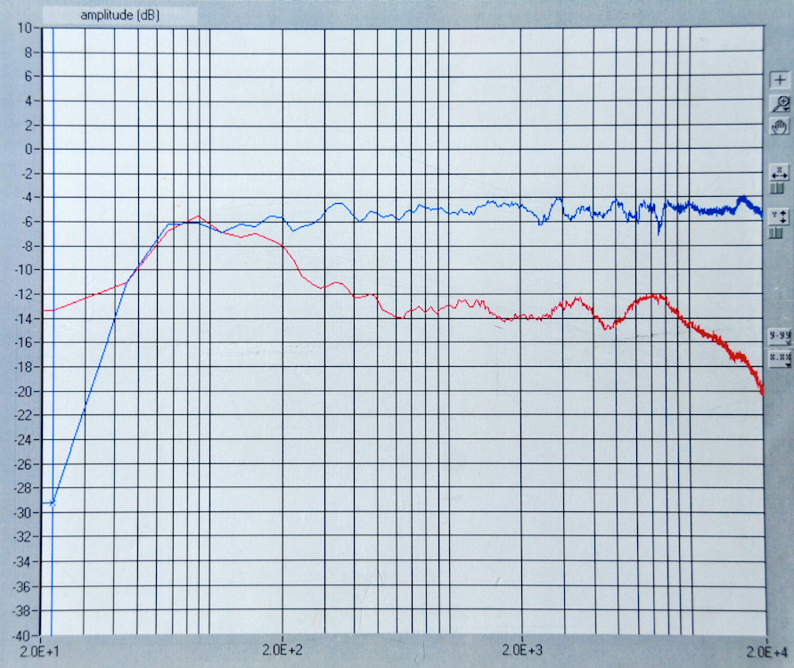
I was part of the development team, and one of the two persons who decided on the final sound design (aka tonal balance) of the B&O H6 headphones. So, I’m happy to share some of the blame for some of the comments (at least on the sound quality) from the reviews.
Audio.de reviewed the H6 paired with an Astell & Kern portable player. They said:
“Tatsächlich aber ertönte der H6 mit dem AK Junior erstaunlich präzise, extrem sauber und stabil und vor allem ungeahnt luftig. Das Zusammenspiel des speziell angefertigten Treibers mit dem ausgeklügelten Bassport stellte nicht etwa – wie oft üblich bei geschlossenen Hörern – die tiefen Frequenzen wummernd und brummend in den Vordergrund. Nein, besonders Stimmen und feine Details profitierten vom knochentrockenen und nicht zu gewaltigen Bass.
“Susanne Sundfos glockenhelle Stimme beispielsweise stand fest gemeißelt im erstaunlich großen Raum, umgeben von jederzeit verfolgbaren Bassdrum-Beats, echten Streichern und Synthesizer-Harmonien. Der kurze Probelauf mit H6 und AK Junior wurde zur ausführlichen Hörsession, die erste Begeisterung zur echten Liebe. Eben true love.”
Correction: That review stated that I said that the H6’s were tuned using the Grado’s as the reference. This is not really true. While we were tuning them, we listened to many different headphones. The Grado’s are one of the many hanging in the listening room…
Gramophone Magazine reviewed the H6 in the April 2014 edition. They said some very nice things about the headphones:
“…excellent clarity and weight, well-defined bass and a sense of openness and space unusual in closed-back headphones. The sound is rich, attractive and ever-so-easy to enjoy.”
and
“… by no means are these headphones designed only for those wanting a pounding bass-line and an exciting overall balance: as already mentioned the bass extension is impressive, but it’s matched with low-end definition and control that’s just as striking, while a smooth midband and airy, but sweet, treble complete the sonic picture.”
and
“As I may have made clear in the past, I haven’t been the greatest fan of headphone listening, much preferring a pair of small speakers on the desk. But with the arrival of fine headphones such as the BeoPlay H6, I’m having to do some re-thinking.”
Bobby Solomon wrote this review at thefoxisblack.com.
“The sound is refined, with the midrange coming through clearly, and the bass and treble are balanced perfectly.”
Kenneth Roberts wrote this review at head-if.org.
“I’d describe B&O’s “house sound” as natural and neutral, with a brilliant, feathery-light high-end that resolves a lot of detail. This describes the H6’s sound perfectly. It delivers a staggering amount of detail in its price-class. In fact, the H6 delivers an impressive amount of detail when compared to headphones well above its price-class! Cymbals, triangles, snares, and hi-hats all sound crisp and light, with nary a hint of sibilance or stridence. I’m guessing this deftly executed high-end lends much to the headphone’s spectacular imaging, which I’ll describe later.”
T3’s website has a review here
“Which rather handily leads us onto how they actually sound. The answer can be summed up with the word ‘balanced’. By this we mean that almost all ranges perform excellently, but never does one take precedence over the other.”
pocketlint.com has their review here
from the middle of the text: “As you might expect, audio quality is top-notch. While we can’t say it competes with some of the other stay-at-home audiophile grade kit, for a set of headphones you can listen to daily, they certainly deliver. Sound is nicely balanced with plenty of detail and not an overly punchy bass. The set of 40mm drivers and the internal bass port just keep everything as clean and simple as possible.”
Tim Gideon and PCMag.com has their review here
The concluding words state: “In the age of big, booming bass, it’s doing its own thing. This is by no means an anemic-sounding headphone pair, it just favors lows, mids, and highs over a wildly boosted sub-bass range. If a more refined, crisp mids-focused sound is what you seek, the H6 will not disappoint, and it’s refreshing to see such a unique sound signature in this field.”
“Bang & Olufsen Finally Got It Right” at head-fi.org
“The sound is surprisingly flat, but a little bit on the warm side. The sound is not as airy as the open back cans, but the soundstage is very good for a portable closed back.”
whathifi.com has a thorough review here
“Based on my favorable impressions of the H6 with the first series of tracks which are heavy on electronic sounds, and also on the second group which feature more conventional bands and acoustic sounds, I’d say the H6 bridges these different genres very well. There are very few headphones that have a decent deep bass response and reasonable impact but don’t have any upper bass emphasis or bloat, and the B&O H6 is one of those few.”
soundandvision.com has a review here
“This is no head-banger headphone, but the bass goes low and it’s nicely articulated. The frequency response is remarkably smooth, without a hint of the rolled highs and boosted bottom common to more mainstream ’phones; the downside to this clarity is that the headphone won’t do anything to blunt the harshness of overcompressed MP3s.”
beforeitsnews.com has a review here
“The sound, however, is near flat and crisp. You’ll be able to hear the fine details of a song or a recording. There’s also no distortion at top volumes, while the midrange is great. Bass is balanced rather than strong, preferring accuracy and refinement to simple power. Think of these headphones as fine wine and other headphones as beers. When you start appreciating its beauty and fine sound, oh boy, where have you been all my life?”
Customer Comments at beoworld.org
There is a long user discussion on the forum here. Persons looking for real-world opinions will certainly get their fill at that site.
“I did not really like the H6 when it was released, a bit thin on an iPhone and a big headphone. And expensive. So I bought the B&W P5 instead. Quite good comfort and good sound. But.. I just had to give the H6 a try so I bought a pair a few days ago (the black model – after a lot of pondering). I now have a completely different feeling about the H6. They sound very natural and good. I like how detailed and precise the sound is. You can hear so many details very well and how acoustic noises changes in frequencies in a wonderful way.”
“My wife has a pair of H6’s in tan, and I am consistently impressed by them.”
“Soundwise, also nice to hear your opinion (and Chris´s). I can’t remember hearing a pair of headphones with a more true sound.”
“I’ve now got a tan pair of my own (240£ for a new pair via eBay) and use them every day. I’ve been listening to some of my favourite music which I’ve listened to for over 40 years on CD, vinyl, digital via an ipod and A8’s and can now pick out musical detail that up to now has eluded me. The separation of instruments on some of my live recordings is incredible, so much so that I’ve found that even Steve Hackett playing live does make some mistakes! None of the music is muddied and I have to say that I don’t find the volume when using an ipod too low. If I want loud music I’ll play it at home on a bigger amp set-up with some bigger speakers. When using the headphones I want the isolation of me and my music.”


