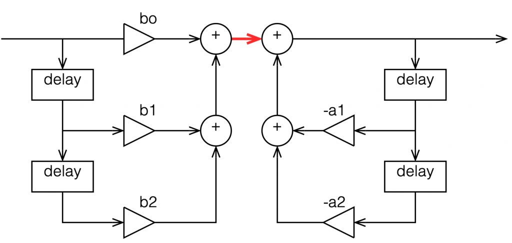
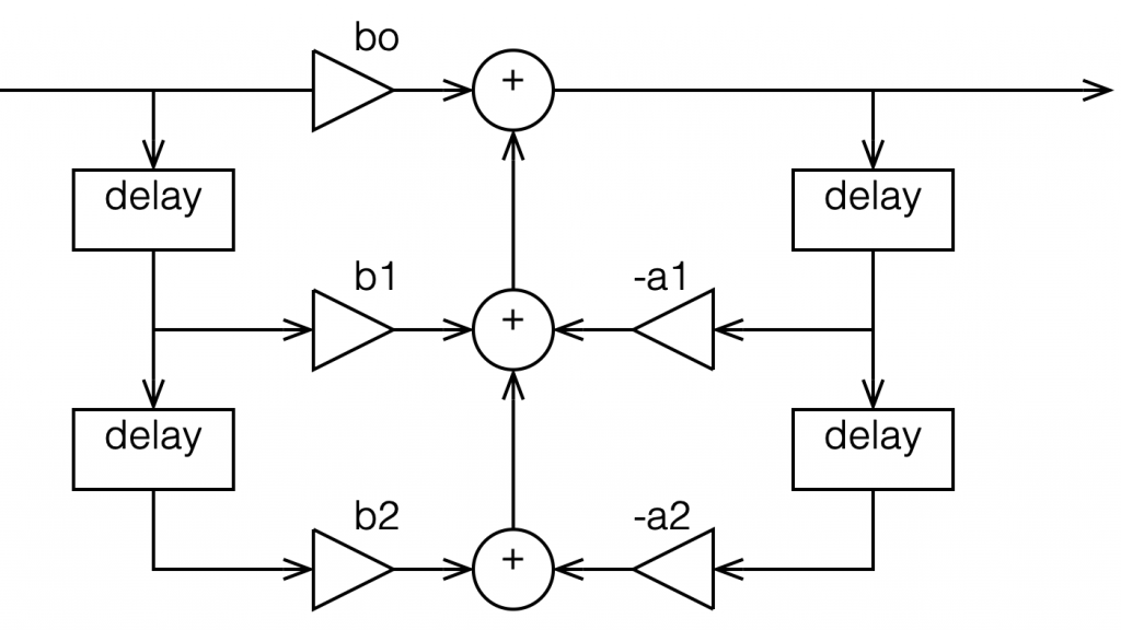
Most digital filters that are applied to audio signals use a “basic” building block called a “biquadratic filter” or “biquad” which consists of 2 feed-forward delays and 2 feed-back delays, each with its own output gain and a delay time of 1 sample. I’ve already talked a little about biquads in this posting, where I showed a couple of different ways to implement it. One of the standard ways is shown below in Figure 1.
The signal flow that I drew for Figure 1 is a little more modular than the way it’s normally shown, but that’s to keep things separate for the purposes of this discussion.
The two feed-forward delays add to the input signal (via gains b0, b1, and b2) and the result shows up at the red arrow. Remember from Part 1 that this portion of the biquad can only make a magnitude response that has (in an extreme case) infinitely deep, sharp dips, and smooth rounded peaks.
The signal from the red arrow onwards goes into the feed-back portion of the filter with two feed-back delays adding through gains -a1 and -a2. Again, remember from Part 1 that this portion of the biquad can make a magnitude response that has infinitely deep, sharp peaks, and smooth rounded dips.
Let’s say that we wanted to make a simple filter – let’s make it a low pass filter – using this biquad. How do we do it?
The simplest way is to cheat and go straight to the answer.
Cheating Option 1: You go to this page at www.earlevel.com and put in the parameters you’re interested in (Filter Type, sampling rate, Fc, Q, etc…) and copy-and-paste the resulting five gains (we’ll call them “coefficients” from now on).
Cheating Option 2: We search on the Interweb for the words “RBJ Audio Cookbook” and then spend some time copying, pasting, and porting the equations that Robert Bristow-Johnson bestowed upon us many years ago* into your processor. You then say “I want a low pass filter at 1000 Hz with a Q of 0.5, please” and the equations spit out the five coefficients that you seek.
However, if you cheat, you’ll never really get a grasp of how those coefficients work and what they’re really doing – and that’s where we’re headed in this little series of articles. So, you might decide to go through this series, and then cheat afterwards (that’s what I would recommend…)
Now, before you go any further, I’ll warn you – the whole purpose of this series is to give you an intuitive understanding. This means that there are things I’m going to (intentionally) skip over, merely mention in passing, or omit completely. So, if you already know what I’m talking about, there’s no point in reading what I’m writing – and there’s certainly no need to email me to remind me that I didn’t mention some aspect of this that you think is important, but I’ve decided is not. If you feel strongly about this, write your own blog.
In the previous posting, we left off with this drawing of a biquad filter:
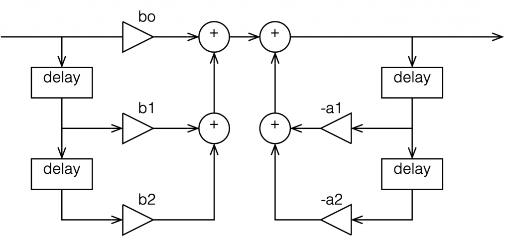
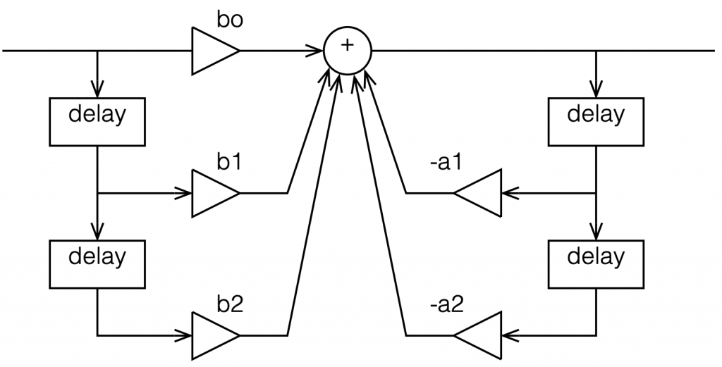
This is not the normal way to draw the signal flow inside a biquad, since it has a little too much information. Normally you see something like this:
or this:
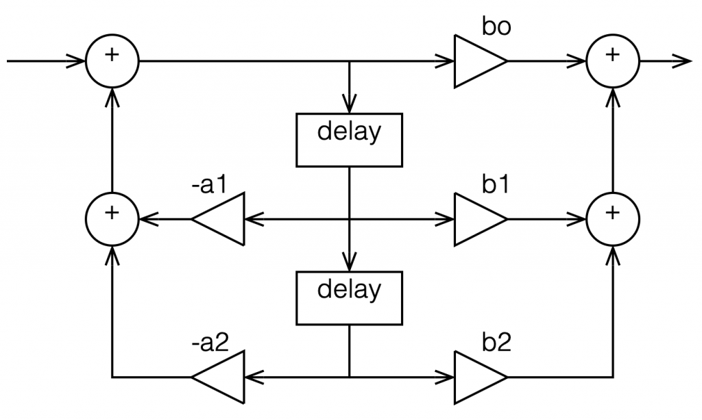
In the versions I show above, the feed-forward half of the biquad comes first, and its output feeds the start of the feedback portion. It is also possible to reverse these, putting the feedback portion first, like this:
In theory, these different implementations will all result in the same output if you match the gain values. However, in practice, they are not the same, and this difference is where we need to look for this part of the discussion on high res audio.
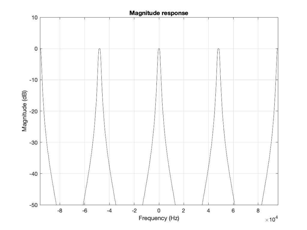
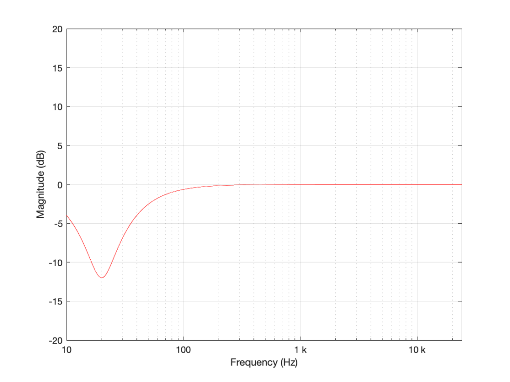
Let’s say I want to make a simple filter that reduces bass in a fairly narrow frequency band. I can use a biquad to do this. For example, if I want a peaking filter that reduces 20 Hz by 12 dB, with a Q of 1, then I get a magnitude response that looks like this:
If I wanted to build this filter using a biquad in a system with a sampling rate of 48 kHz, it would have the following gain coefficients:
We’ll also say that my biquad is implemented like the one shown in Figure 1, above… let’s take a look at that signal flow again:
I’ve highlighted a point inside the biquad using a red arrow. Let’s talk about the signal right there, in the middle of the processing…
In the last post, we talked about how, when the signal frequency is very low, a single sample delay has almost the same value at its output as its input, because the phase difference is so small for such a small time. So, let’s start with the (incorrect) assumption that, for those two feed-forward delays at the beginning, their outputs ARE equal to their inputs (because we’re starting with a low frequency). What happens when the input has a value of 1? Then the value at the red arrow is just the sum of the feed forward gains (because I multiplied each of them by 1 and added them together…)
In the case of the filter I described above, this value will be 0.000006836, which is a very small number. Also, if the value coming into the input of the biquad is less than 1, the value at the red arrow will be even smaller! This means that, if you come into the biquad with a low-frequency tone with a level of 0 dB FS, the level at that red arrow will be about -103 dB FS, which is very quiet. The feed-back portion of the biquad, after the red arrow, then has a lot of gain in it to bring the signal level back up towards 0 dB FS again.
So, the issue that we have here is that the FF (Feed Forward) portion of the biquad drops the level A LOT. And the FB portion increases the level A LOT, just to do something like a little 12 dB dip at 20 Hz.
The magnitude of the gains downwards and upwards in those two portions of the biquad are dependent on the parameters of the filter that we’re trying to make, however, we can generalise a little and say that:
the lower the frequency OR
the higher the Q,
then the bigger the gain down and up.
In other words, if you have a really low frequency dip, with a really high Q, then the level of the signal at that red arrow will be really low. REALLY low.
How low can you go?
How low is “REALLY low”? let’s see:
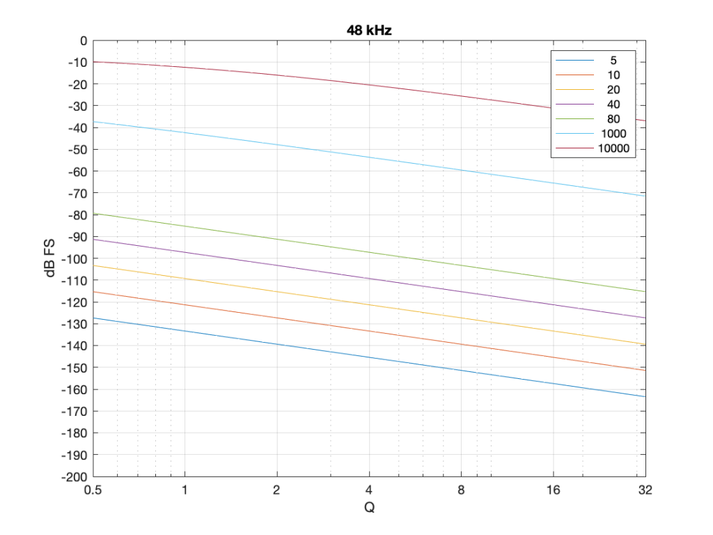
Take a look at Figure 7, which shows some values for one example filter (peaking, Gain = -12 dB, variable Q and Fc, and the test frequency = Fc). Notice that when the Fc is 10 kHz, even at earn Q=32, the signal level at the middle of the biquad is about -38 dB FS or so. However, when the Fc is 20 Hz, it’s -140 dB FS… This is very low.
Now let’s try again at a higher sampling rate: 192 kHz.
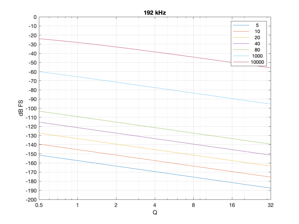
Notice that when we do exactly the same thing running at 192 kHz, the signal levels inside the biquad get much lower. Now for a 20 Hz signal and a Q of 32, the level is around -163 dB FS – a drop of more than 20 dB for 4x the sampling rate.
Why does this happen? It’s because the filter doesn’t “know” that the signal is at 20 Hz. It only knows the relationship between the frequency and the sampling rate. So, in its little world, 20 Hz doesn’t exist. In a system running at 48 kHz, what exists is 20 / 48000 = 0.0004167. This is called the “normalised frequency” where the sampling rate is 1, DC is 0, and everything else is in between. (Note that some textbooks and software say that Nyquist = 1 instead of the sampling rate – but you just need to know what the convention is for the thing you’re reading…) This means that if the sampling rate goes up to 192 kHz, then the normalised frequency for 20 Hz is 20 / 192000 = 0.0001042 (1/4 of the value because the sampling rate was multiplied by 4).
So what?
This is important. If you want to make a low-frequency, high-Q peaking filter in a digital system with a cut of 12 dB, you are forcing the signal to a very low level inside your filter, and then bringing it back up to a normal level again on the way out. If your processing is running with a limited resolution, (e.g. 16-bits, for example) then the signal level can approach or even go below the resolution of your system inside the biquad. This means that, when the signal’s level is raised again on the way out, it’s full of quantisation distortion, and you can’t get rid of it… This is bad.
There are different ways to solve this problem.
Increase the resolution of your processing internally. For example, even though your input and output might only be running at 16-bits or 24-bits, maybe you need more resolution inside to make the results of the math better – or at least below the limitations of the input and output.
Change the way the biquad is implemented. For example, if you use the implementation shown in Figure 4 (with the feedback before the feed-forward) instead of the one we used, then you don’t drop the signal level and raise it again, you do the opposite. This avoids your quantisation error problem. However, depending on the system, it might overload and clip the signal inside the biquad instead, so then you just end up with a different kind of distortion instead.
Reduce your sampling rate to make it closer to your filter’s frequency. The problem I showed above is that the centre frequency of the filter is too far away from the sampling rate. If the sampling rate were lower, then this automatically makes the filter’s centre frequency “higher” in a normalised frequency scale, thus reducing the problem.
Other, even more clever solutions that I won’t talk about because they’re not as simple.
This means (for example) that if you’re building a subwoofer with digital filtering, and you know for sure that NOTHING will come out of it above, say 1 kHz (just to pick a random number that’s far enough away from the typical 120 Hz that people normally use…) then it would be dumb to do the filtering at 192 kHz. It’s smarter to run its internal sampling rate at 2 kHz (because we only need to go up to 1 kHz; and we’re not considering anything other issues or artefacts in this posting.)
P.S.
For this discussion, I used the specific example of a peaking filter with a gain of -12 dB, and I was varying the Q and the Fc. I was also measuring the level of the signal using a sine wave with a frequency that was the same as Fc in each case. However, the general lesson here about low frequency and high-Q filtering holds for other filter types and implementations as well.
Today I was working on a little acoustics simulation patcher in Cycling 74’s Max, and part of the code required the use of a modulo function. No problem, right?
Problem. I originally wrote the code in Matlab, and I was porting it to Max; and the numbers just weren’t working properly. After getting rid of my own home-made bugs, it still wasn’t working…
Turns out that there seems to be a disagreement in the code community about how to do the modulo of a negative number.
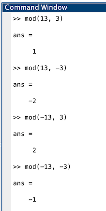
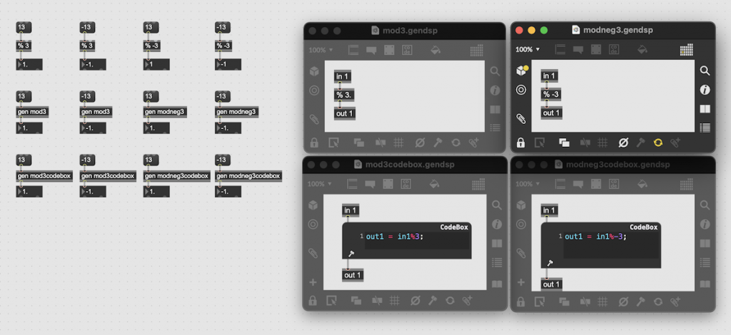
The best indication of the problem I was facing is found on this page, where you can see that different languages come up with different answers for -13 mod 3 and 13 mod -3. The problem is that neither Max nor Matlab are in the list. So: here are the results of those two, to add to the list.
The results are:
Language
13 mod 3
-13 mod 3
13 mod -3
-13 mod -13
Matlab
1
2
-2
-1
Max
1
-1
1
-1
This means that Matlab behaves like Python, using the formula
mod(a, n) = a – n * floor(a / n)
whereas Max behaves like C and Java.
So, if you, like me, move back and forth between Matlab and Max, beware!
#1: You have to drive to a meet someone at a specific time. Let’s say that you only have to drive on one road to get there, and the speed limit is the same the whole way. You calculate the time it will take to get there on time, and you start driving – but there’s traffic. So, you wind up driving half the distance at half the speed, then the traffic disappears.
How fast do you have to go the rest of the way to arrive at the meeting on time?
#2: You’re driving on a two-lane highway where the speed limit is 70 km/h. You are driving 100 km/h, and you pull into the left lane to pass someone who is driving the speed limit. Everything about the car you’re passing is identical to yours – even the driver weighs the same as you do. At the instant that you are side-by side, a train appears across the road in front of you and stops. You both hit the brakes at exactly the same time to try and stop from hitting the train.
Luckily, the person in the other car stops just as his bumper touches the train, let’s say 1 mm before touching it… But, because you were driving faster, you cannot stop in time.
How fast are you going when you hit the train?
The answers
#1. Most people instinctively say “double the speed limit” to make up the lost time. However, this is not the right answer.
Let’s say that the meeting is 100 km away, and the speed limit is 100 km/h. Therefore, it should take you 1 hour to get to the meeting.
If you drive half the distance (50 km) at half the speed (50 km/h), then at the moment the traffic clears up, you should have been at your destination. So, you would have to drive infinity km/h to get there. However, since teleportation doesn’t exist yet, you might as well just call and tell them you’ll be late.
#2: This one is a little tougher, but it should be pretty intuitive for someone working in audio. A car’s brakes work by taking the energy in the car’s momentum, and converting that to heat in the brake discs. The key word there is energy.
So, the question is: if you consider the amount of energy removed from the car going 70 km/h, and take that out of the energy in the car going 100 km/h, how much energy is left?
The answer is 70 km/h. For someone in audio, this might look like a familiar answer, since 0.7 V has half of the power of 1.0 V (assuming identical loads). In the case of the cars, it’s because the amount of power (the amount of energy that’s transmitted over time – in this case, to heat the brakes) to bring the car from 70 km/h to 0 km/h is identical to the amount of power it takes to bring the same car from 100 km/h to 70 km/h. (An audio geek might joke that 70 km/h is 3 dB slower than 100 km/h.)
The conclusion
Slow down. You’re not going to make it to the meeting anyway, and driving a little bit faster means you’re going to hit the train much harder than you think.
These days, I’m spending a lot of time wrapping my head around the relationship between the frequency and the time responses of filters. In doing so, I’m digging into the concept of “Q”, of course. As a result, I’m reading my old books and some Internet sites, and I’m frequently presented with something like the following:
That, of course, is from the Wikipedia entry on “Q”.
However, in the Bell Telephone System Technical Publication – Monograph 2491, called “The Story of Q” by Estill I. Green ( published in the American Scientist, Vol 43, pp 584-594, in October 1955), it states:
“For a time, Johnson* designated the ratio of reactance to effective resistance of a coil by the symbol K. It was in 1920, while working the practical application of the wave filter which G. A. Campbell had invented some years before, that he for the first time employed the symbol Q for his parameter. His reason for choosing Q was quite simple. He says that it did not stand for ‘quality factor’ or anything else, but since the other letters of the alphabet had already been pre-empted for other purposes, Q was all he had left.”
So, if we’re going to be pedantic (which I love to be) there are two errors on that Wikipedia page. Firstly, Q does not stand for Quality. Secondly, it’s not the “Q factor”, it’s just the “Q”.
As an aside, that monograph is not only informative, it’s fun to read (depending, of course, on your definition of “fun”). For example, near the end of the paper, Green applies Q to rotating bodies (which is not a surprise, since an audio-wave oscillation is just a rotation represented in two dimensions). In that section, he points out that the rotation of the earth is slowing down due, in part, to tidal friction. Consequently, the length of a day is increasing at a rate of 0.00164 second per century, which would make the Q of the rotation of the earth equal to about 10,000,000,000,000 (10^13).
* K.S. Johnson worked in the Western Electric Company’s Engineering Department, which became Bell Telephone Laboratories in 1925.
This week, I was asked a very specific question about connecting an older pair of Beolab loudspeakers to a stereo preamp from another company. Specifically, the owner was wondering why the pairing wasn’t working out too well – and he had already had a theory that the problem had something to do with the sensitivity of his Beolab 9’s.
To be honest, I don’t really know what the problem is with this specific customer’s system – but I made a guess and I figured that the answer might be useful to someone else…
For starters, let’s do some sensitivity training. More accurately, let’s talk about loudspeaker sensitivity. This is a measure of how loud the acoustical output of a loudspeaker is for a given electrical input. Since Beolab loudspeakers are active (meaning, in part, that the amplifiers are built-in) this means that we are talking about an output level in dB SPL for a given input in volts.
For most Beolab loudspeakers, you will get an output of 88 dB SPL for an input of 125 mV RMS if you measure the loudspeaker on-axis in a free field. There are some exceptions to this, most notably Beolab 1, 9, and 5, which will produce 91 dB SPL instead.
So, this tells us how loud the loudspeaker will be for a given input. But my guess is that this had nothing to do with the customer’s problem.
Most customers connect their Beolab loudspeakers to a Bang & Olufsen source using something called a “Power Link” connection. This is a little bundle of wires that contains two audio channels (probably left and right) as well as a data channel (telling the loudspeaker things like the volume setting, for example) and a 5 V DC on/off signal.
Power Link is specified to have a maximum level of 6.5 V RMS, assuming that the signal is a sine wave. This means that a device with a Power Link output can produce no more than 9.2 V Peak. It also means that a device with a Power Link input (like a Beolab loudspeaker) will clip (and therefore distort) at its input if you feed it with more than 9.2 V Peak.
(If you do some math, you can calculate that 20*log10(6.5 V RMS / 125 mV RMS) = 34.3 dB. Therefore, if a Beolab 9 loudspeaker will produce 91 dB SPL with a 125 mV RMS input, then it should produce 91+34.3 dB = 125.3 dB SPL for a maximum accepted input of 6.5 V RMS. Of course, this is not possible – but it’s because the loudspeaker is limited by its drivers, amplifiers, and power supply – not the input maximum input level.)
Back to the question: The customer in question mentioned his stereo preamp’s brand and model number. A little Duck-Duck-Go-ing helped me to find the manual for that particular device, and in the back of that document, I found out that the maximum output level of the preamp was 29 V RMS – which is a lot…
So, the problem is very likely that his preamp is overloading the input stages of the Beolab 9. So, if he turns the volume knob on the preamp up to maximum, and he’s playing a tune that is mastered to be loud on the playback media, then the Beolab 9’s input will be clipped. Changing the sensitivity of the loudspeaker could make it quieter – but it will still be clipped… So the distortion won’t get better – everything will just get quieter.
There are some different solutions to this problem. The easiest one is to not turn up the volume on the preamp – but this is not the best solution, because it means that he’s not using the full dynamic range of the preamp (probably), and therefore that the noise from the preamp is higher in level than it needs to be at the input of the Beolab 9.
There is, however, a very cheap and simple solution, and that is to attenuate the output of the preamp so that when it is set to its maximum output level, it is just hitting the maximum input level of the loudspeaker’s input.
How do we do this? the first question is to find out what the attenuation should be.
Maximum output level = 29.0 V RMS
Maximum input level = 6.5 V RMS
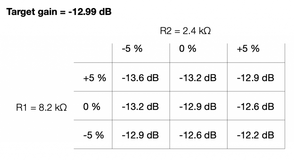
20*log10 (6.5 / 29.0) = -12.99 dB
This is the same as a linear gain of 0.2241.
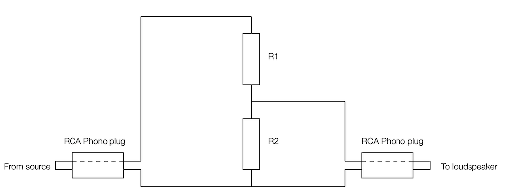
Now we’re going to build a voltage divider. This is device made of two resistors, placed in series (end-to-end) and connected to the output of the source. The point where the two resistors connect together is used as the output to the loudspeaker, resulting in a schematic as shown below.
As you can probably see in the schematic, the grounds of the two devices (which are connected to the exterior casings of the RCA Phono plugs) are connected together. As the voltage on the pin of the source goes up and down, the voltage on the pin of the loudspeaker also goes up and down – but by less. How much less is determined by the values of the resistors.
For example, if the resistors are equal (R1 = R2) then the output will be half of the input. If R2 is one tenth of the total of R1+R2, then the output will be one tenth of the input. You can calculate this gain yourself with a simple equation:
Linear Gain = R2 / (R1 + R2)
and
Gain in dB = 20 * log10 (Linear Gain)
So, for example, if R1 = 8,000 Ω and R2 = 2,000 Ω, then the gain will be
2000 / (8000 + 2000) = 0.2
which is equal to 20*log10 (0.2) -13.98 dB.
Unfortunately, if you want to do this with only two resistors, you can’t be too choosy about their resistances. There are standard resistor values, and you’ll have to pick from that list.
Also, it’s a good “rule of thumb” to try and keep the resistance “seen” by the source around 10,000 Ω (or 10 kΩ) – just to keep it happy. If you make the value too low, then you will be asking for it to deliver too much current (and its maximum output level will drop). If you make it too high, you might create and antenna and result in some extra noise…
So, I want to make R1 +R2 about 10,000 Ω, and I want R2 / (R1+R2) to be about 0.2241 (because I’m trying to convert 29 V RMS to 6.5 V RMS). So, I go to a list of standard resistor values like this one and I start trying to simultaneously fulfill those two requirements.
After some trial and error, I find out that if I make R1 = 8.2 kΩ and R2 = 2.4 kΩ, I can come pretty close.
2400 / (8200 + 2400) = 0.2264 = -12.902
close enough. Now I just need to get a soldering iron and a bit of wire, and put it all together…
The details…
However, if you clicked on that list of standard resistor values, you might notice that it says ±5% at the top of the table. This is normal. If you go to your local resistor store and you buy a 1 kΩ resistor – it probably won’t be exactly 1,000.000000000 Ω. But it will be close. If you buy from the ±5% stack, then any resistor in that bunch will be within 5% of the stated value. So, for a 1 kΩ resistor ±5%, it will be somewhere between 950 Ω and 1050 Ω.
So, then the question is, for the resistors that I just picked, how bad can it get, and is that good enough?
Well… this can be calculated. I just put in the worst-case values for my two resistors into the math, and do it over and over until I get all the possible answers. This would look like this:
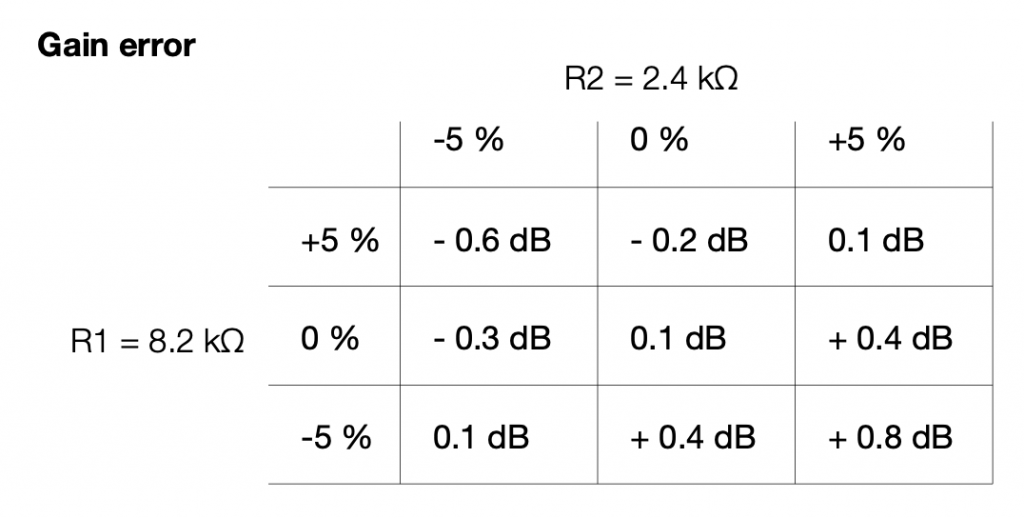
If we look at this in terms of how far away we are from the target – the gain error, then it looks like this:
So, if we randomly choose resistors out of the bag, the worst that can happen is that we will be 0.6 dB below the target or 0.8 dB above the target.
This means that, if we’re not careful, and we’re unlucky, then we can get a mismatch between the two channels of 1.4 dB (assuming that one channel was a worst-case low and the other is a worst-case high). This is enough to be audible as about a 15% shift towards the louder loudspeaker, which is probably not acceptable.
So, the moral of the story is that you should measure your resistors before soldering them into the circuit.
Note, however, that it’s not necessary to make the gains perfect to improve the imaging. You just need to make them equal in the two channels for that…
Speaking Passively
The circuit I show above is called a “passive” circuit. This means that it doesn’t require any external power source (like a battery or a power supply) to work. However, it also means that it can’t make things louder – no matter what resistor values you choose, the output will always be less than the input.
There are lots of reasons why this is a useful little circuit. It’s cheap, it’s easy to make, it’s small (you could hide it inside one of the RCA connectors), and it will prevent you from overloading the input of the downstream device (in this case, a loudspeaker). Not only that, but it will also attenuate the noise generated by the source – so not only will the customer’s system no longer clip, it will also (probably) have a lower noise floor.