Category: perception
Data visualisation
This past week, I spent two days learning the basics of representing data in Tableau, which led to a discussion about Stephen Few, who has some opinions about clearly representing your data.
That, in turn, got me thinking about one of my old hobby horses – my personal mission to eliminate the world of spider plots.
Human Echolocation
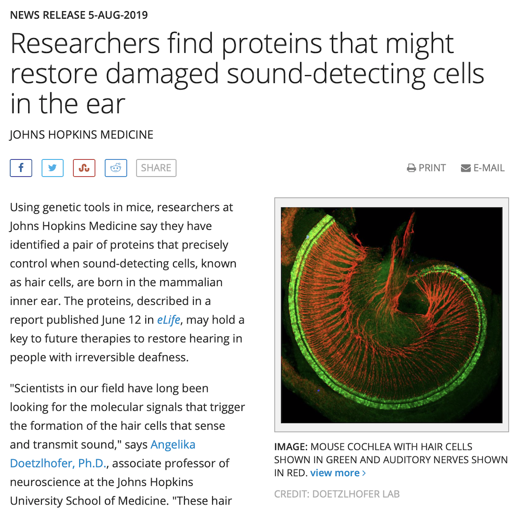
A little good news
(don’t) Listen to this…
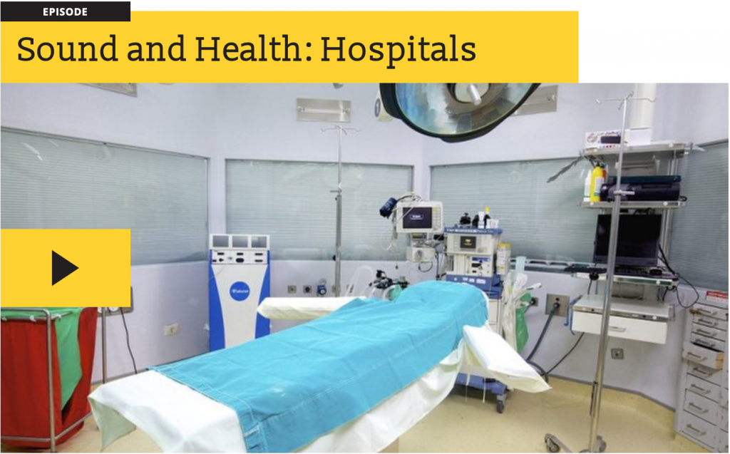
A two-part excellent podcast on the effects of sound on our health.

Immersive audio
Typical Errors in Digital Audio: Part 8 – The Weakest Link
As a setup for this posting, I have to start with some background information…
Back when I was doing my bachelor’s of music degree, I used to make some pocket money playing background music for things like wedding receptions. One of the good things about playing such a gig was that, for the most part, no one is listening to you… You’re just filling in as part of the background noise. So, as the evening went on, and I grew more and more tired, I would change to simpler and simpler arrangements of the tunes. Leaving some notes out meant I didn’t have to think as quickly, and, since no one was really listening, I could get away with it.
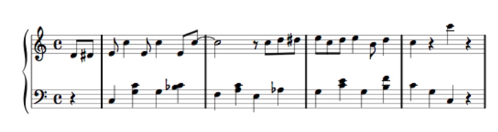
If you watch the short video above, you’ll hear the same composition played 3 times (the 4th is just a copy of the first, for comparison). The first arrangement contains a total of 71 notes, as shown below.

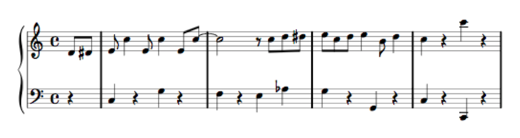
The second arrangement uses only 38 notes, as you can see in Figure 2, below.
The third arrangement uses even fewer notes – a total of only 27 notes, shown in Figure 3, below.
The point of this story is that, in all three arrangements, the piece of music is easily recognisable. And, if it’s late in the night and you’ve had too much to drink at the wedding reception, I’d probably get away with not playing the full arrangement without you even noticing the difference…
A psychoacoustic CODEC (Compression DECompression) algorithm works in a very similar way. I’ll explain…
If you do an “audiometry test”, you’ll be put in a very, very quiet room and given a pair of headphones and a button. in an adjacent room is a person who sees a light when you press the button and controls a tone generator. You’ll be told that you’ll hear a tone in one ear from the headphones, and when you do, you should push the button. When you do this, the tone will get quieter, and you’ll push the button again. This will happen over and over until you can’t hear the tone. This is repeated in your two ears at different frequencies (and, of course, the whole thing is randomised so that you can’t predict a response…)
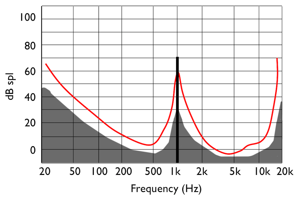
If you do this test, and if you have textbook-quality hearing, then you’ll find out that your threshold of hearing is different at different frequencies. In fact, a plot of the quietest tones you can hear at different frequencies it will look something like that shown in Figure 4.
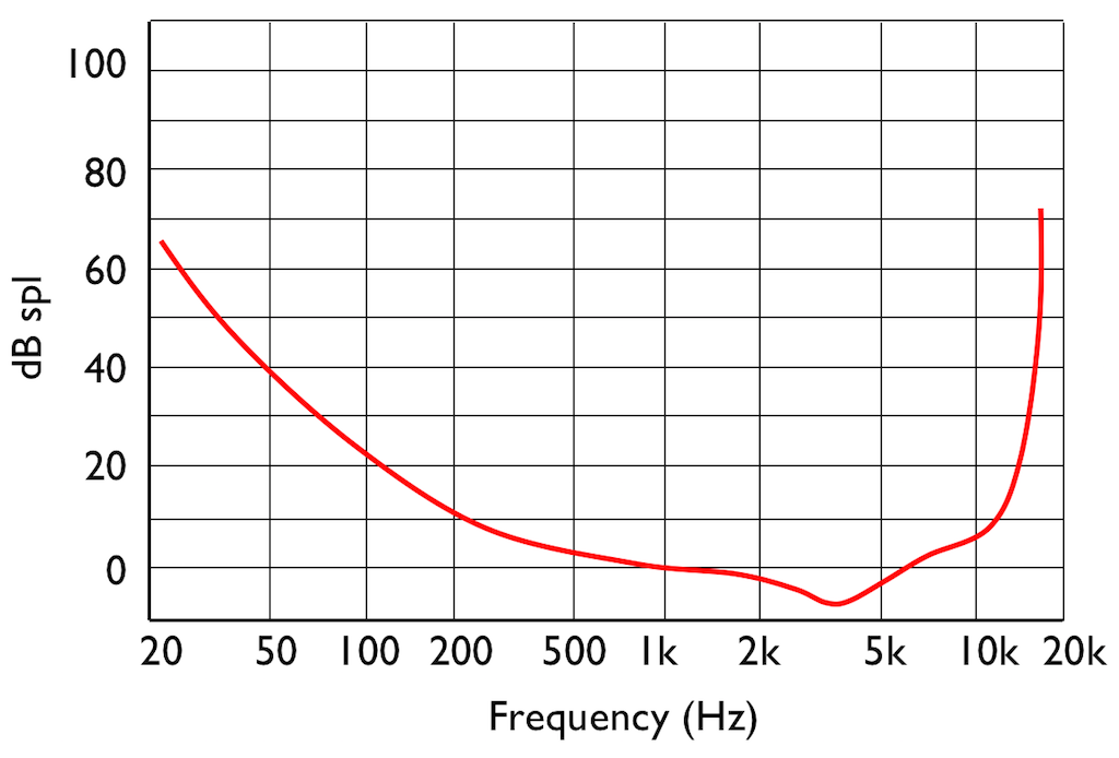
This red curve shows a typical curve for a threshold of hearing. Any frequency that was played at a level that would be below this red curve would not be audible. Note that the threshold is very different at different frequencies.

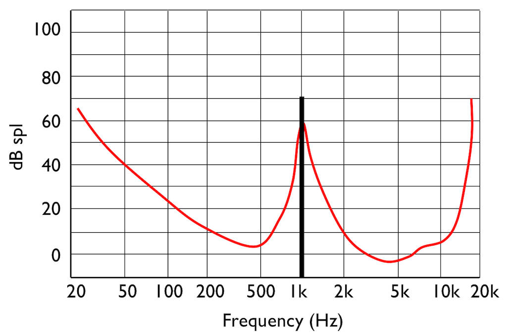
Interestingly, if you do play this tone shown in Figure 5, then your threshold of hearing will change, as is shown in Figure 6.
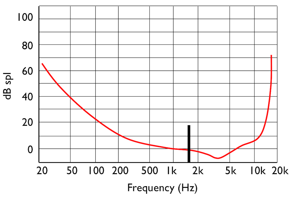
IF you were not playing that loud 1 kHz tone, and, instead, you played a quieter tone just below 2 kHz, it would also be audible, since it’s also above the threshold of hearing (shown in Figure 7.
However, if you play those two tones simultaneously, what happens?
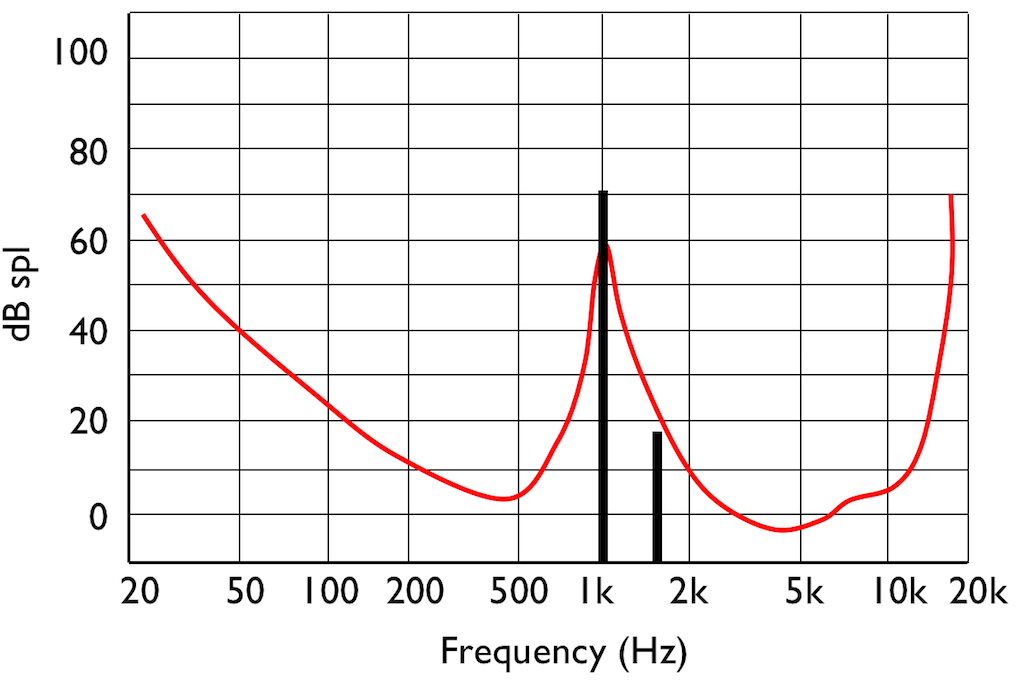
This effect is called “psychoacoustic masking” – the quieter tone is masked by the louder tone if the two area reasonably close together in frequency. This is essentially the same reason that you can’t hear someone whispering to you at an AC/DC concert… Normal people call it being “drowned out” by the guitar solo. Scientists will call it “psychoacoustic masking”.
Let’s pull these two stories together… The reason I started leaving notes out when I was playing background music was that my processing power was getting limited (because I was getting tired) and the people listening weren’t able to tell the difference. This is how I got away with it. Of course, if you were listening, you would have noticed – but that’s just a chance I had to take.
If you want to record, store, or transmit an audio signal and you don’t have enough processing power, storage area, or bandwidth, you need to leave stuff out. There are lots of strategies for doing this – but one of them is to get a computer to analyse the frequency content of the signal and try to predict what components of the signal will be psychoacoustically masked and leave those components out. So, essentially, just like I was trying to predict which notes you wouldn’t miss, a computer is trying to predict what you won’t be able to hear…
This process is a general description of what is done in all the psychoacoustic CODECs like MP3, Ogg Vorbis, AC-3, AAC, SBC, and so on and so on. These are all called “lossy” CODECs because some components of the audio signal are lost in the encoding process. Of course, these CODECs have different perceived qualities because they all have different prediction algorithms, and some are better at predicting what you can’t hear than others. Also, depending on what bitrate is available, the algorithms may be more or less aggressive in making their decisions about your abilities.
There’s just one small problem… If you remove some components of the audio signal, then you create an error, and the creation of that error generates noise. However, the algorithm has an trick up its sleeve. It knows the error it has created, it knows the frequency content of the signal that it’s keeping (and therefore it knows the resulting elevated masking threshold). So it uses that “knowledge” to shape the frequency spectrum of the error to sit under the resulting threshold of hearing, as shown by the gray area in Figure 9.
Let’s assume that this system works. (In fact, some of the algorithms work very well, if you consider how much data is being eliminated… There’s no need to be snobbish…)
Now to the real part of the story…
Okay – everything above was just the “setup” for this posting.
For this test, I put two .wav files on a NAS drive. Both files had a sampling rate of 48 kHz, one file was a 16-bit file and the other was a 24-bit file.
On the NAS drive, I have two different applications that act as audio servers. These two applications come from two different companies, and each one has an associated “player” app that I’ve put on my phone. However, the app on the phone is really just acting as a remote control in this case.
The two audio server applications on the NAS drive are able to stream via my 2.4 GHz WiFi to an audio device acting as a receiver. I captured the output from that receiver playing the two files using the two server applications. (therefore there were 4 tests run)
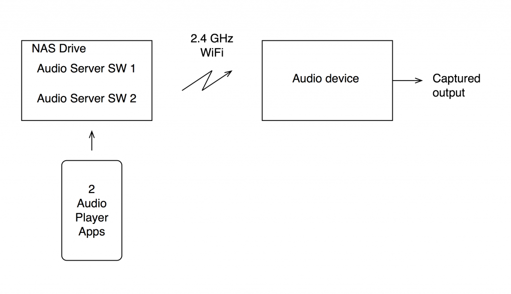
The content of the signal in the two .wav files was a swept sine tone, going from 20 Hz to 90% of Nyquist, at 0 dB FS. I captured the output of the audio device in Figure 10 and ran a spectrogram of the result, analysing the signal down to 100 dB below the signal’s level. The results are shown below.
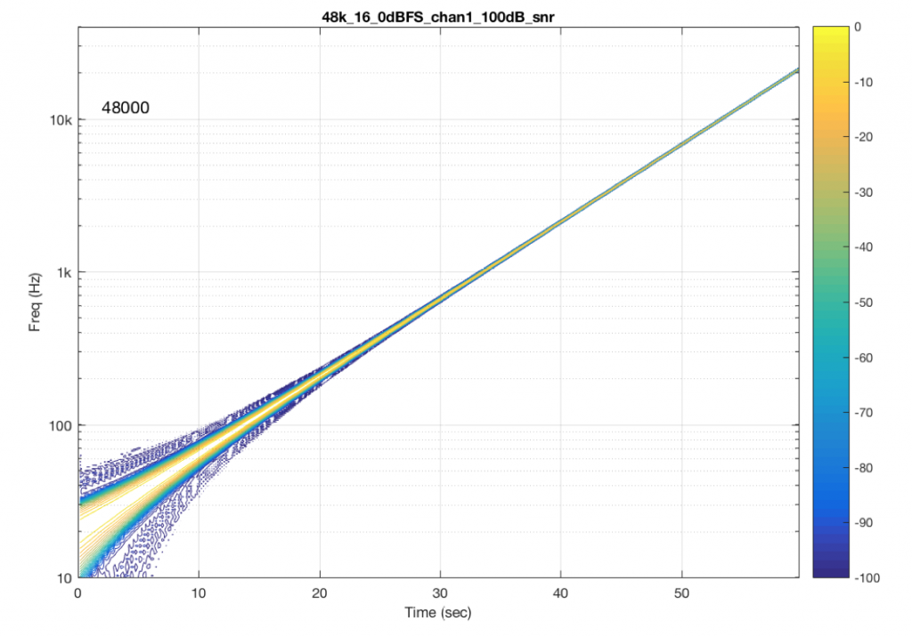


So, Figures 11 and 13 show the same file (the 16-bit version) played to the same output device over the same network, using two different audio server applications on my NAS drive.
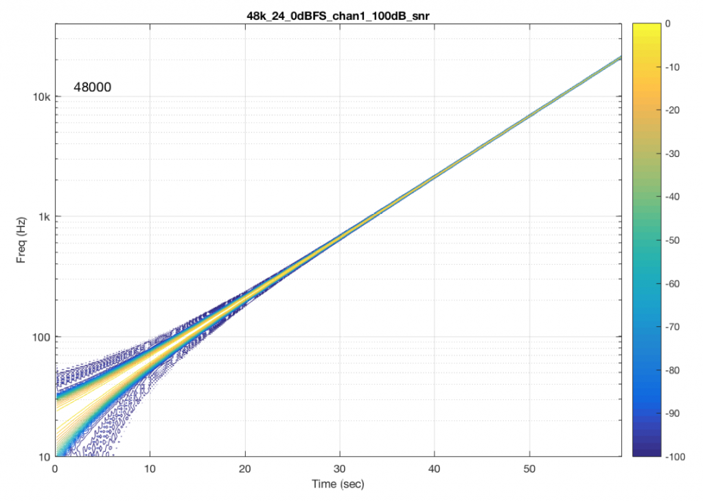
Figures 12 and 14 also show the same file (the 24-bit version). As is immediately obvious, the “Audio Server SW 2” is not nearly as happy about playing the 24-bit file. There is harmonic distortion (the diagonal lines parallel with the signal), probably caused by clipping. This also generates aliasing, as we saw in a previous posting.
However, there is also a lot of visible noise around the signal – the “fuzzy blobs” that surround the signal. This has the same appearance as what you would see from the output of a psychoacoustic CODEC – it’s the noise that the encoder tries to “fit under” the signal, as shown in Figure 9… One give-away that this is probably the case is that the vertical width (the frequency spread) of that noise appears to be much wider when the signal is a low-frequency. This is because this plot has a logarithmic frequency scale, but a CODEC encoder “thinks” on a linear frequency scale. So, frequency bands of equal widths on a linear scale will appear to be wider in the low end on a log scale. (Another way to think of this is that there are as many “Hertz’s” from 0 Hz to 10 kHz as there are from 10 kHz to 20 kHz. The width of both of these bands is 10000 Hz. However, those of us who are still young enough to hear up there will only hear the second of these as the top octave – and there are lots of octaves in the first one. (I know, if we go all the way to 0 Hz, then there are an infinite number of octaves, but I don’t want to discuss Zeno today…))
Conclusion
So, it appears that “Audio Server SW 2” on my NAS drive doesn’t like sending 24 bits directly to my audio device. Instead, it probably decodes the wav file, and transcodes the lossless LPCM format into a lossy CODEC (clipping the signal in the process) and sends that instead. So, by playing a “high resolution” audio file using that application, I get poorer quality at the output.
As always, I’m not going to discuss whether this effect is audible or not. That’s irrelevant, since it’s dependent on too many other factors.
And, as always, I’m not going to put brand or model names on any of the software or hardware tested here. If, for no other reason, this is because this problem may have already been corrected in a firmware update that has come out since I tested it.
The take-home messages here are:
- an entire audio signal path can be brought down by one piece of software in the audio chain
- you can’t test a system with one audio file and assume that it will work for all other sampling rates, bit depths and formats
- Normally, when I run this test, I do it for all combinations of 6 sampling rates, 2 bit depths, and 2 formats (WAV and FLAC), at at least 2 different signal levels – meaning 48 tests per DUT
- What I often see is that a system that is “bit perfect” in one format / sampling rate / bit depth is not necessarily behaving in another, as I showed above..
So, if you read a test involving a particular NAS drive, or a particular Audio Server application, or a particular audio device using a file format with a sampling rate and a bit depth and the reviewer says “This system worked perfectly.” You cannot assume that your system will also work perfectly unless all aspects of your system are identical to the tested system. Changing one link in the chain (even upgrading the software version) can wreck everything…
This makes life confusing, unfortunately. However, it does mean that, if someone sounds wrong to you with your own system, there’s no need to chase down excruciating minutiae like how many nanoseconds of jitter you have at your DAC’s input, or whether the cat sleeping on your amplifier is absorbing enough cosmic rays. It could be because your high-res file is getting clipped, aliased, and converted to MP3 before sending to your speakers…
Addendum
Just in case you’re wondering, I tested these two systems above with all 6 standard sampling rates (44.1, 48, 88.2, 96, 176.4, and 192 kHz), 2 bit depths (16 & 24). I also did two formats (WAV and FLAC) and three signal levels (0, -1, and -60 dB FS) – although that doesn’t matter for this last comment.
“Audio Server SW 2” had the same behaviour in the case of all sampling rates – 16 bit files played without artefacts within 100 dB of the 0 dB FS signal, whereas 24-bit files in all sampling rates exhibited the same errors as are shown in Figure 14.
One way to compare CODEC quality
I’m often asked about my opinion regarding sound quality vs. compression formats or sampling rates or bit depths or psychoacoustic CODEC’s or other things like that…
Of course, there are lots of ways to decide on such an opinion, depending on what parameters you use to define “sound quality” and therefore what it is you’re asking specifically…
One way to think of this is to consider that the original sound file is the “reference” (regardless of how “good” or “bad” it is…), and when you encode it somehow (say, by changing sampling rates, or making it an MP3 file, for example), AND that encoding makes it different, then the resulting difference from the original can be considered an error.
So, I took a compilation of tracks that I often use for listening to loudspeakers. This is about 13 minutes long and is made of excerpts of many different recordings and recording styles, ranging from anechoic female speech, through a cappella choral, orchestral music, jazz, hard rock, heavy metal, and hip hop. The original tracks were all taken from 44.1 kHz / 16-bit CD’s, and the compilation is a 44.1 kHz / 16 bit result. This is what we’ll call the “reference”.
I then used LAME to encode the compilation in different bitrates of MP3. I re-encoded as 320, 256, and 128 CBR (Constant Bit Rate). I also used the “–preset” option to make encodings in the “insane”, “extreme”, “standard”, and “medium” settings (I’ve included the details of this at the bottom in the “Appendix”). Three of these four presets are VBR – the “Insane” setting is a CBR 320 kbps with some tweaked parameters.
I decoded those MP3 files back to PCM, and compared them to the original, of course making sure that everything was time- and gain-aligned. (There are some small differences in the overall level of the original file and the MP3 output – which is different for different bitrates. If I did not do this, then I would be exaggerating the differences between the original and the encoded versions – so this gain difference was calculated and compensated for, before subtracting the original from the MP3.)
Let’s take a look at a plot of the sample values in the left channel of the beginning of the track.
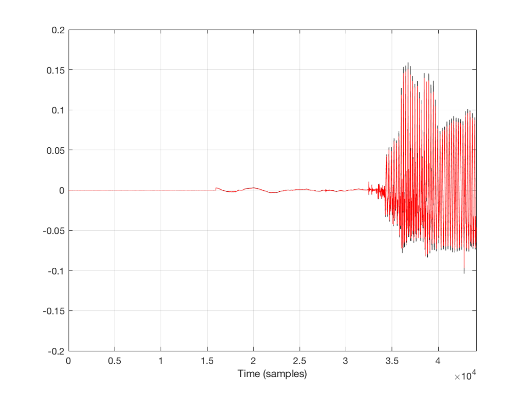
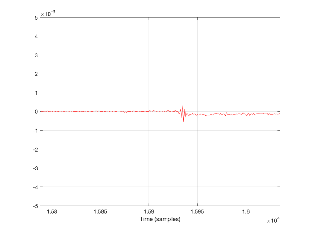
The plot above shows the first 44100 samples in the track (the first second of sound). The red plot is the decoded 128 kbps MP3. The black plot (which is difficult to see because it is overlapped by the red plot – except in the signal peaks) is the original file. For example, if I zoom into the area around the beginning of the sound (say, starting around sample number 15800) then we see this

So, as you can see in the two plots above, the decoded 128 kbps MP3 and the original 44.1/16 file are different. But, the difference is small relative to the levels of the signals themselves. The question is, how small is the difference, exactly?
We can find this out by subtracting the original signal from the decoded MP3 output, sample by sample. The result of this is shown in the plot below.
Notice that the vertical scale of the plot in Figure 3 is small. This is because it shows the difference between the two lines in Figure 2, which is also quite small.
Let’s think for a minute about how I arrived at the signal in Figure 3. I subtracted the Original signal from the MP3 output. In other words:
MP3 output – Original = Difference
If we consider that the difference between the MP3 output and the Original can be thought of as an “error”, and if I move the terms in the equation above, I get the following:
MP3 output – Original = Error
Original + Error = MP3 output
So, the question is: how loud is that error relative to the signal we’re listening to? The idea here is that, the louder the error, the easier it will be to detect.
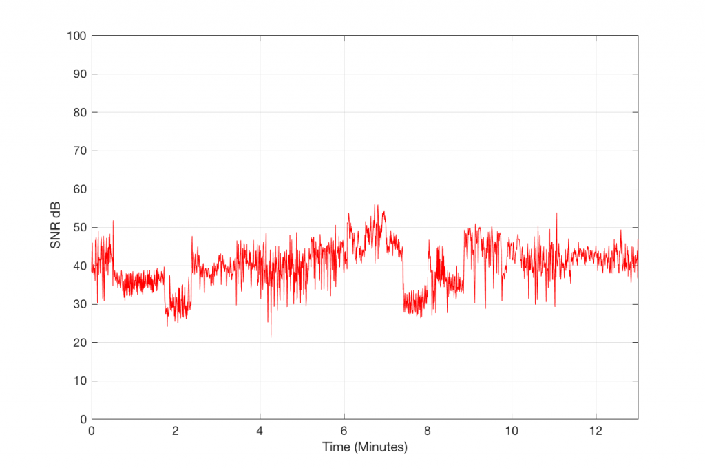
Figure 4, below, shows this level difference over time. The black curve is a running RMS level of the decoded 128 kbps MP3 file. As you can see there, it ranges from about -30 dB FS to about +10 dB FS. You may think that it’s strange that it “only” goes to -10 dB FS – but this is because the time window I’m using to calculate the RMS value of the signal is 500 ms long. The peaks of the track reach full scale, but since my time window is long, this tends to pull down the apparent level (because the peaks are short). (NB: If you want to argue about the choice of a 500 ms time window, please wait until I’ve followed up this posting with another one that divides things up by frequency band…)
The res curve in Figure 4 is a running RMS value of the Error signal – the difference between the MP3 file and the original. As you can see there, that error signal ranges from about -50 dB FS to about -30 dB FS, give or take…
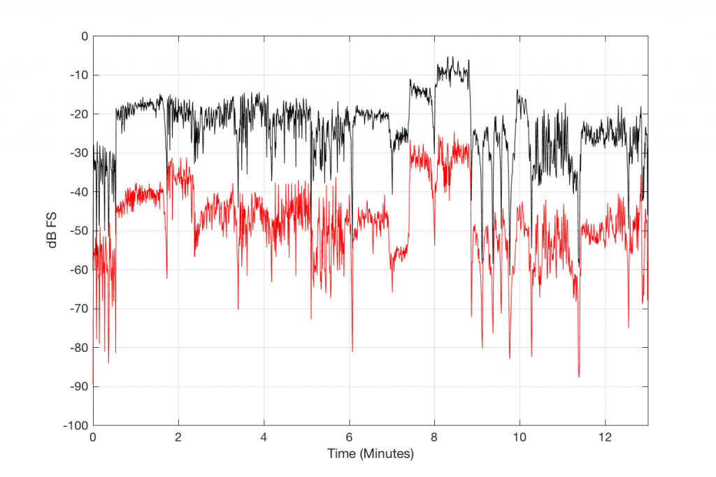
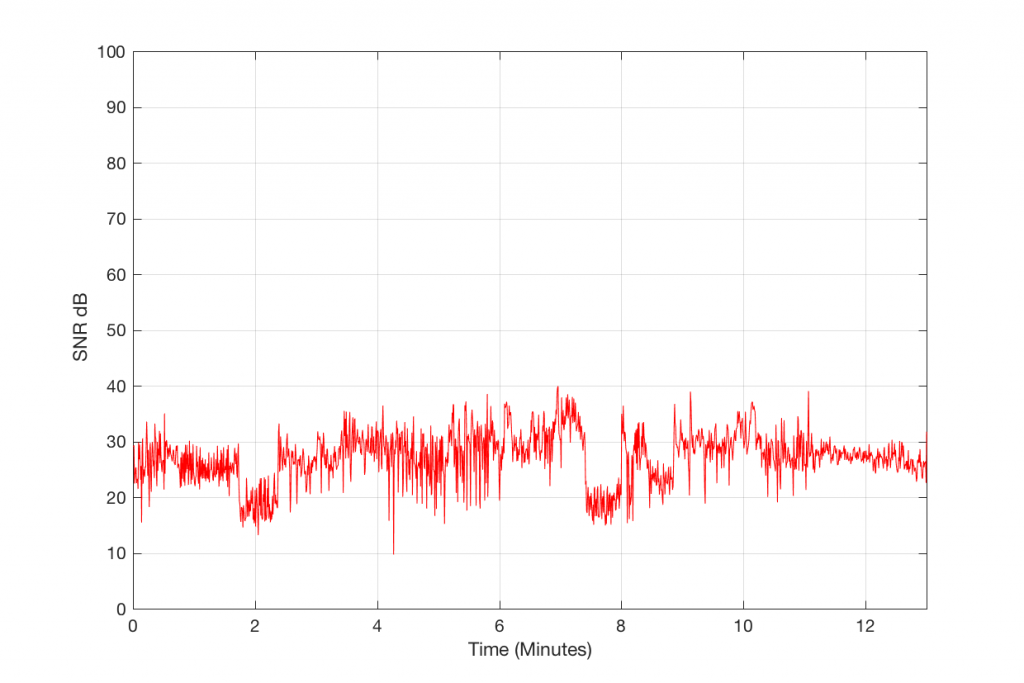
We can find the running value of the difference between the level of the MP3 file and the level of the Error it contains by subtracting the black curve from the red curve. The result of this is shown in Figure 5, below.

So, Figure 5, therefore, shows the measure of how loud the signal is relative to the error that makes it different from the original. If this error signal were just harmonic distortion, then we could call this a measure of THD in dB. If it were just good-old-fashioned noise, like on a magnetic tape, then we could call it a signal-to-noise ratio. However, this is neither distortion or noise in the traditional sense – or, maybe more accurately, it’s both…
So, let’s call the plot in Figure 5 a “signal-to-error ratio”. What we can see there is that, for this particular track, for the settings that I used to make the 128 kbps MP3 file, the error – the MP3 artefacts – are only 20 to 25 dB below the signal most of the time. Now, don’t jump to conclusions here. This does not mean that they would be as audible as white noise that is only 25 dB below the signal. This is because part of the “magic” of the MP3 encoder is that it tries to ensure that the error can “hide” under the signal by placing the error signal in the same frequency band(s) as the signal. Typically, white noise is in a different band than the signal, so it’s easier to hear because it’s not masked. So, be very careful about interpreting this plot. This is a measurable signal-to-error ratio, but it cannot be directly compared to a signal-to-noise ratio.
Let’s now increase the bitrate of the MP3 encoding, allowing the encoder to increase the quality.


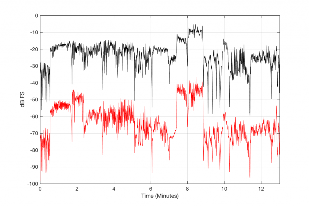
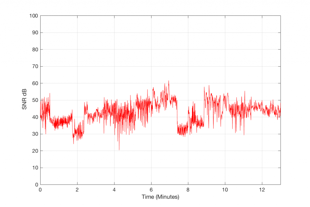
Figure 6 and 7 show the same information as before, but for a 256 kpbs encoding of the same track. As you can see there, by doubling the bitrate of the MP3, we have increased our signal-to-error ratio by about 10 to 15 dB or so – to about 35 or 40 dB.
As you can see in Figures 8 and 9 above, increasing the MP3 bitrate to 320 kbps can improve the Signal-to-Error ratio from about 25 dB (for 128 kbps) to about 40 dB or so.
Now, if you’re looking carefully, you might notice that, some times in the track that I used for testing, the signal-to-error ratio is actually worse for the 320 kbps file than it is for the 256 kbps file – all other things being equal in the LAME converter parameters. This is a bit misleading, since what you cannot see there is the frequency spectrum of the error signal. I’ll deal with that in a future posting – with some more analysis and explanation to go with it.
For now, let’s play with the VBR presets in LAME. I’ll just show the signal-to-error plots for the 4 settings.


So, as you can see in Figures 10 through 13, the signal-to-error ratio can be improved with the VBR presets, reaching a peak of over 60 dB for the “Insane” setting, for this track…
As I said a couple of times above:
- You have to be careful about interpreting these graphs from a background of “knowing” what a SNR is… This error is not normal “distortion” or “noise” – at least from a perceptual point of view…
- I’ll go further with this, including some frequency-dependent information in a future posting.
Appendix – LAME parameters and verbose output
For the geeks…
MAC60090:mp3_demos ggm$ lame -b 320 -q 0 –verbose compilation_original.wav lame_320.mp3
LAME 3.99.5 64bits (http://lame.sf.net)
Using polyphase lowpass filter, transition band: 20094 Hz – 20627 Hz
Encoding compilation_original.wav to lame_320.mp3
Encoding as 44.1 kHz j-stereo MPEG-1 Layer III (4.4x) 320 kbps qval=0
misc:
scaling: 1
ch0 (left) scaling: 1
ch1 (right) scaling: 1
huffman search: best (outside loop)
experimental Y=0
…
stream format:
MPEG-1 Layer 3
2 channel – joint stereo
padding: off
constant bitrate – CBR
using LAME Tag
…
psychoacoustic:
using short blocks: channel coupled
subblock gain: 1
adjust masking: -10 dB
adjust masking short: -11 dB
quantization comparison: 9
^ comparison short blocks: 9
noise shaping: 1
^ amplification: 2
^ stopping: 1
ATH: using
^ type: 4
^ shape: 0 (only for type 4)
^ level adjustement: -12 dB
^ adjust type: 3
^ adjust sensitivity power: 1.000000
experimental psy tunings by Naoki Shibata
adjust masking bass=-0.5 dB, alto=-0.25 dB, treble=-0.025 dB, sfb21=0.5 dB
using temporal masking effect: yes
interchannel masking ratio: 0
…
Frame | CPU time/estim | REAL time/estim | play/CPU | ETA
37028/37028 (100%)| 2:07/ 2:07| 2:08/ 2:08| 7.5929x| 0:00
————————————————————————————————–
kbps LR MS % long switch short %
320.0 73.7 26.3 93.4 3.4 3.1
Writing LAME Tag…done
ReplayGain: -2.6dB
MAC60090:mp3_demos ggm$ lame -b 256 -q 0 –verbose compilation_original.wav lame_256.mp3
LAME 3.99.5 64bits (http://lame.sf.net)
Using polyphase lowpass filter, transition band: 19383 Hz – 19916 Hz
Encoding compilation_original.wav to lame_256.mp3
Encoding as 44.1 kHz j-stereo MPEG-1 Layer III (5.5x) 256 kbps qval=0
misc:
scaling: 1
ch0 (left) scaling: 1
ch1 (right) scaling: 1
huffman search: best (outside loop)
experimental Y=0
…
stream format:
MPEG-1 Layer 3
2 channel – joint stereo
padding: off
constant bitrate – CBR
using LAME Tag
…
psychoacoustic:
using short blocks: channel coupled
subblock gain: 1
adjust masking: -8 dB
adjust masking short: -8.8 dB
quantization comparison: 9
^ comparison short blocks: 9
noise shaping: 1
^ amplification: 2
^ stopping: 1
ATH: using
^ type: 4
^ shape: 1 (only for type 4)
^ level adjustement: -10 dB
^ adjust type: 3
^ adjust sensitivity power: 1.000000
experimental psy tunings by Naoki Shibata
adjust masking bass=-0.5 dB, alto=-0.25 dB, treble=-0.025 dB, sfb21=0.5 dB
using temporal masking effect: yes
interchannel masking ratio: 0
…
Frame | CPU time/estim | REAL time/estim | play/CPU | ETA
37028/37028 (100%)| 1:50/ 1:50| 1:51/ 1:51| 8.7235x| 0:00
————————————————————————————————–
kbps LR MS % long switch short %
256.0 71.6 28.4 93.4 3.4 3.1
Writing LAME Tag…done
ReplayGain: -2.6dB
MAC60090:mp3_demos ggm$ lame -b 128 -q 0 –verbose compilation_original.wav lame_128.mp3
LAME 3.99.5 64bits (http://lame.sf.net)
Using polyphase lowpass filter, transition band: 16538 Hz – 17071 Hz
Encoding compilation_original.wav to lame_128.mp3
Encoding as 44.1 kHz j-stereo MPEG-1 Layer III (11x) 128 kbps qval=0
misc:
scaling: 0.95
ch0 (left) scaling: 1
ch1 (right) scaling: 1
huffman search: best (outside loop)
experimental Y=0
…
stream format:
MPEG-1 Layer 3
2 channel – joint stereo
padding: off
constant bitrate – CBR
using LAME Tag
…
psychoacoustic:
using short blocks: channel coupled
subblock gain: 1
adjust masking: 0 dB
adjust masking short: 0 dB
quantization comparison: 9
^ comparison short blocks: 9
noise shaping: 2
^ amplification: 2
^ stopping: 1
ATH: using
^ type: 4
^ shape: 4 (only for type 4)
^ level adjustement: -3 dB
^ adjust type: 3
^ adjust sensitivity power: 1.000000
experimental psy tunings by Naoki Shibata
adjust masking bass=-0.5 dB, alto=-0.25 dB, treble=-0.025 dB, sfb21=0.5 dB
using temporal masking effect: yes
interchannel masking ratio: 0.0002
…
Frame | CPU time/estim | REAL time/estim | play/CPU | ETA
37028/37028 (100%)| 1:33/ 1:33| 1:34/ 1:34| 10.305x| 0:00
————————————————————————————————–
kbps LR MS % long switch short %
128.0 25.2 74.8 95.2 2.6 2.2
Writing LAME Tag…done
ReplayGain: -2.2dB
MAC60090:mp3_demos ggm$ lame –preset medium –verbose compilation_original.wav lame_medium.mp3
LAME 3.99.5 64bits (http://lame.sf.net)
Using polyphase lowpass filter, transition band: 17249 Hz – 17782 Hz
Encoding compilation_original.wav to lame_medium.mp3
Encoding as 44.1 kHz j-stereo MPEG-1 Layer III VBR(q=4)
misc:
scaling: 1
ch0 (left) scaling: 1
ch1 (right) scaling: 1
huffman search: best (outside loop)
experimental Y=1
…
stream format:
MPEG-1 Layer 3
2 channel – joint stereo
padding: all
variable bitrate – VBR mtrh (default)
using LAME Tag
…
psychoacoustic:
using short blocks: channel coupled
subblock gain: 1
adjust masking: 0 dB
adjust masking short: 0 dB
quantization comparison: 9
^ comparison short blocks: 9
noise shaping: 1
^ amplification: 2
^ stopping: 1
ATH: using
^ type: 5
^ shape: 2 (only for type 4)
^ level adjustement: -0 dB
^ adjust type: 3
^ adjust sensitivity power: 6.309574
experimental psy tunings by Naoki Shibata
adjust masking bass=-0.5 dB, alto=-0.25 dB, treble=-0.025 dB, sfb21=3.5 dB
using temporal masking effect: no
interchannel masking ratio: 0
…
Frame | CPU time/estim | REAL time/estim | play/CPU | ETA
37028/37028 (100%)| 0:18/ 0:18| 0:19/ 0:19| 53.116x| 0:00
32 [ 37] %
40 [ 4] *
48 [ 14] %
56 [ 8] %
64 [ 105] %
80 [ 423] %*
96 [ 831] %***
112 [ 2596] %%%********
128 [17134] %%%%%%%%%%%%%%%%%%%%***********************************************
160 [12811] %%%%%%%%%%%%%%%%%%%%%%%%***************************
192 [ 1330] %%****
224 [ 836] %%**
256 [ 683] %**
320 [ 216] %
——————————————————————————-
kbps LR MS % long switch short %
144.3 35.5 64.5 90.7 4.6 4.7
Writing LAME Tag…done
ReplayGain: -2.6dB
MAC60090:mp3_demos ggm$ lame –preset standard –verbose compilation_original.wav lame_standard.mp3
LAME 3.99.5 64bits (http://lame.sf.net)
Using polyphase lowpass filter, transition band: 18671 Hz – 19205 Hz
Encoding compilation_original.wav to lame_standard.mp3
Encoding as 44.1 kHz j-stereo MPEG-1 Layer III VBR(q=2)
misc:
scaling: 1
ch0 (left) scaling: 1
ch1 (right) scaling: 1
huffman search: best (outside loop)
experimental Y=0
…
stream format:
MPEG-1 Layer 3
2 channel – joint stereo
padding: all
variable bitrate – VBR mtrh (default)
using LAME Tag
…
psychoacoustic:
using short blocks: channel coupled
subblock gain: 1
adjust masking: -2.6 dB
adjust masking short: -2.6 dB
quantization comparison: 9
^ comparison short blocks: 9
noise shaping: 1
^ amplification: 2
^ stopping: 1
ATH: using
^ type: 5
^ shape: 2 (only for type 4)
^ level adjustement: -3.7 dB
^ adjust type: 3
^ adjust sensitivity power: 1.995262
experimental psy tunings by Naoki Shibata
adjust masking bass=-0.5 dB, alto=-0.25 dB, treble=-0.025 dB, sfb21=6.25 dB
using temporal masking effect: no
interchannel masking ratio: 0
…
Frame | CPU time/estim | REAL time/estim | play/CPU | ETA
37028/37028 (100%)| 0:19/ 0:19| 0:20/ 0:20| 48.732x| 0:00
32 [ 0]
40 [ 0]
48 [ 1] %
56 [ 0]
64 [ 15] %
80 [ 26] %
96 [ 17] %
112 [ 135] %
128 [ 1673] %*******
160 [15048] %%%%%%%%%%%%%%%%%%%%%%%%%%%%%%%%%%%%*****************************
192 [15688] %%%%%%%%%%%%%%%%%%%%%%%%%%%%%%%%%%%%%%%%%%%%%%%%%%*****************
224 [ 1986] %%%%%****
256 [ 1602] %%%%***
320 [ 837] %%**
——————————————————————————-
kbps LR MS % long switch short %
183.0 60.0 40.0 90.7 4.6 4.7
Writing LAME Tag…done
ReplayGain: -2.6dB
MAC60090:mp3_demos ggm$ lame –preset extreme –verbose compilation_original.wav lame_extreme.mp3
LAME 3.99.5 64bits (http://lame.sf.net)
polyphase lowpass filter disabled
Encoding compilation_original.wav to lame_extreme.mp3
Encoding as 44.1 kHz j-stereo MPEG-1 Layer III VBR(q=0)
misc:
scaling: 1
ch0 (left) scaling: 1
ch1 (right) scaling: 1
huffman search: best (outside loop)
experimental Y=0
…
stream format:
MPEG-1 Layer 3
2 channel – joint stereo
padding: all
variable bitrate – VBR mtrh (default)
using LAME Tag
…
psychoacoustic:
using short blocks: channel coupled
subblock gain: 1
adjust masking: -6.8 dB
adjust masking short: -6.8 dB
quantization comparison: 9
^ comparison short blocks: 9
noise shaping: 1
^ amplification: 2
^ stopping: 1
ATH: using
^ type: 5
^ shape: 1 (only for type 4)
^ level adjustement: -7.1 dB
^ adjust type: 3
^ adjust sensitivity power: 1.000000
experimental psy tunings by Naoki Shibata
adjust masking bass=-0.5 dB, alto=-0.25 dB, treble=-0.025 dB, sfb21=8.25 dB
using temporal masking effect: no
interchannel masking ratio: 0
…
Frame | CPU time/estim | REAL time/estim | play/CPU | ETA
37028/37028 (100%)| 0:21/ 0:21| 0:22/ 0:22| 44.584x| 0:00
32 [ 0]
40 [ 0]
48 [ 0]
56 [ 0]
64 [ 0]
80 [ 0]
96 [ 0]
112 [ 1] %
128 [ 0]
160 [ 408] %*
192 [ 1961] %%******
224 [16481] %%%%%%%%%%%%%%%%%%%%%%%%%%%%%%%%%%%%%%%%%%%%%%%%%%%%***************
256 [13387] %%%%%%%%%%%%%%%%%%%%%%%%%%%%%%%%%%%%%%%%%%*************
320 [ 4790] %%%%%%%%%%%%%*******
——————————————————————————-
kbps LR MS % long switch short %
245.6 70.9 29.1 90.7 4.6 4.7
Writing LAME Tag…done
ReplayGain: -2.6dB
MAC60090:mp3_demos ggm$ lame –preset insane –verbose compilation_original.wav lame_insane.mp3
LAME 3.99.5 64bits (http://lame.sf.net)
Using polyphase lowpass filter, transition band: 20094 Hz – 20627 Hz
Encoding compilation_original.wav to lame_insane.mp3
Encoding as 44.1 kHz j-stereo MPEG-1 Layer III (4.4x) 320 kbps qval=3
misc:
scaling: 1
ch0 (left) scaling: 1
ch1 (right) scaling: 1
huffman search: best (outside loop)
experimental Y=0
…
stream format:
MPEG-1 Layer 3
2 channel – joint stereo
padding: off
constant bitrate – CBR
using LAME Tag
…
psychoacoustic:
using short blocks: channel coupled
subblock gain: 1
adjust masking: -10 dB
adjust masking short: -11 dB
quantization comparison: 9
^ comparison short blocks: 9
noise shaping: 1
^ amplification: 1
^ stopping: 1
ATH: using
^ type: 4
^ shape: 0 (only for type 4)
^ level adjustement: -12 dB
^ adjust type: 3
^ adjust sensitivity power: 1.000000
experimental psy tunings by Naoki Shibata
adjust masking bass=-0.5 dB, alto=-0.25 dB, treble=-0.025 dB, sfb21=0.5 dB
using temporal masking effect: yes
interchannel masking ratio: 0
…
Frame | CPU time/estim | REAL time/estim | play/CPU | ETA
37028/37028 (100%)| 0:28/ 0:28| 0:28/ 0:28| 33.937x| 0:00
——————————————————————————-
kbps LR MS % long switch short %
320.0 73.7 26.3 93.4 3.4 3.1
Writing LAME Tag…done
ReplayGain: -2.6dB
Modern acoustical design

B&O Tech: “Auto” loudness
#76 in a series of articles about the technology behind Bang & Olufsen loudspeakers
If you look at the comments section to a posting I wrote about ABL, you’ll see a short conversation there between me and a happy Beomaster 8000 customer who said that I had made an error in making sweeping generalisations about the function of a “loudness” filter in older gear. I said that, in older gear, a loudness filter boosted the bass (and maybe the treble) with a fixed gain, regardless of listening level (also known as “the position of the volume knob”). Henning said that this was incorrect, and that, in his Beomaster 8000, the amount of boost applied by the loudness filter was, indeed, varied with volume.
So, I dusted off one of our Beomaster 8000’s (made in the early 1980’s) to find out if he was correct.
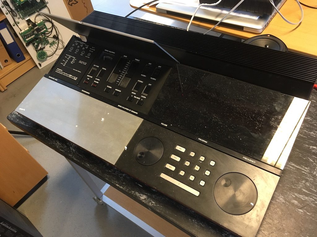
I sent an MLS signal to the Tape 1 input (left channel) of the Beomaster 8000, and connected a differential probe to the speaker output. (The reason for the probe was to bring the signal back down to something like a line level to keep my sound card happy…)
I set the volume to 0.1, switched the loudness filter off, and measured the magnitude response.
Then I turned the loudness filter on, and measured again.
I repeated this for volume steps 0.5, 1.0, 1.5, 2.0, 2.5, 3.0, 3.5, 4.0, 4.5, 5.0, and 5.5. I didn’t do volume step 6.0 because this overloaded the input of my sound card and created the weird artefacts that occur when you clip an MLS signal. No matter…
Then I plotted the results, which are shown below.

Remember that these are NOT the absolute magnitude response curves of the Beomaster 8000. These are the DIFFERENCE between the Loudness ON and Loudness OFF at different volume settings.
At the top, you see a green line which is very, very flat. This means that, at the highest volume setting I tested (vol = 5.5) there was no difference between loudness on and off.
As you start coming down, you can see that the bass is boosted more and more, starting even at volume step 5.0 (the purple line, second from the top). At the bottom volume step (0.1, there is a nearly 35 dB boost at 20 Hz when the loudness filter is on.
You may also notice two other things in these plots. The first is the ripple in the lower curves. the second is the apparent treble boost at the bottom setting. Both of these artefacts are not actually in the signal. These are artefacts of the measurements that I did. So, you should ignore them, since they’re not there in “real life”.
So, Henning, I was wrong and you are correct – the Beomaster 8000 does indeed have a loudness filter that varies with volume. I stand corrected. Thanks for the info – and a fun afternoon!