#73 in a series of articles about the technology behind Bang & Olufsen loudspeakers
The setup
Let’s start by inventing a loudspeaker. It has a perfectly flat on-axis response in a free field. This means that if you send a signal into it, then it doesn’t cause any particular frequency to sound louder or quieter than the others when you measure it in an infinite space that is free of reflections.
We’ll also say that it has a perfectly omnidirectional directivity. This means that the loudspeaker has the same behaviour in all directions – there is no “front” or “back” – sound goes everywhere identically.
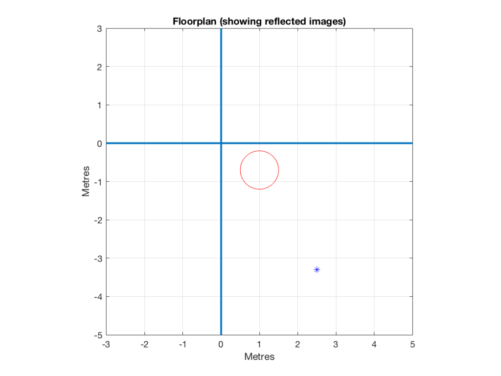
Let’s then put that loudspeaker in a strange room that has only two walls – the left wall and the front wall – and these extend to infinity. We’ll put the loudspeaker, say 1 m from the left wall and 70 cm from the front wall. These are completely arbitrary values, but they’re not weird… Finally, we’ll sit 3 m away from the loudspeaker, as if we were set up to listen to it as the left front loudspeaker in a stereo pair.
A floorpan of that setup is shown below in Figure 1.
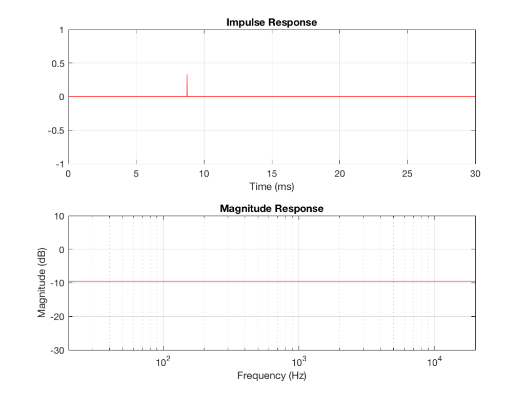
If the two walls were completely absorptive, then there would be no energy reflected from them. If we were to replace the loudspeaker with a light bulb, then the equivalent would be to paint the walls flat black so no light would be reflected. In this theoretically perfect case, then the impulse response and the magnitude response of the loudspeaker at the listening position would be the same as in a free field, since there are no reflections. These would look like the plots in Figure 2.
Through the looking glass
Imagine that you’re standing outdoors on a moonless night, and the only things you have with you are a lightbulb (that is magically lit) and a mirror. You’ll be able to see two light bulbs – the real one, and the one that is reflected by the mirror. If there is really no other light and no other objects, then you won’t even know that it’s a mirror, and you’ll just see two light bulbs (unless, of course, you can see yourself as well…)
In 1929, an acoustical physicist working at Bell Laboratories named Carl F. Eyring presented a new idea to the Acoustical Society of America. He was trying to calculate the reverberation time in “dead” rooms by considering that the walls were perfect mirrors, and that instead of thinking of sound sources and reflections, you could just pretend that the walls didn’t exist, and that the reflections were actually just images of other sound sources on the other side of the wall (just like that second light bulb in the example above…)
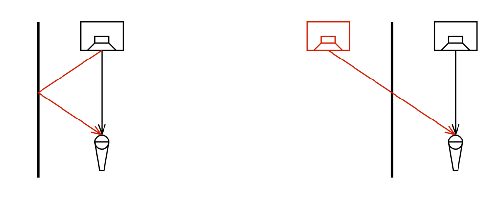
This method of simulating and predicting acoustical behaviour in rooms, now called the “image model” has been used by many people over the decades. Eyring published a paper describing it in 1930, but it has since been standard method, both for prediction and acoustical simulation (first proposed by Allen and Berkley in 1979).
The effects of one sidewall reflection
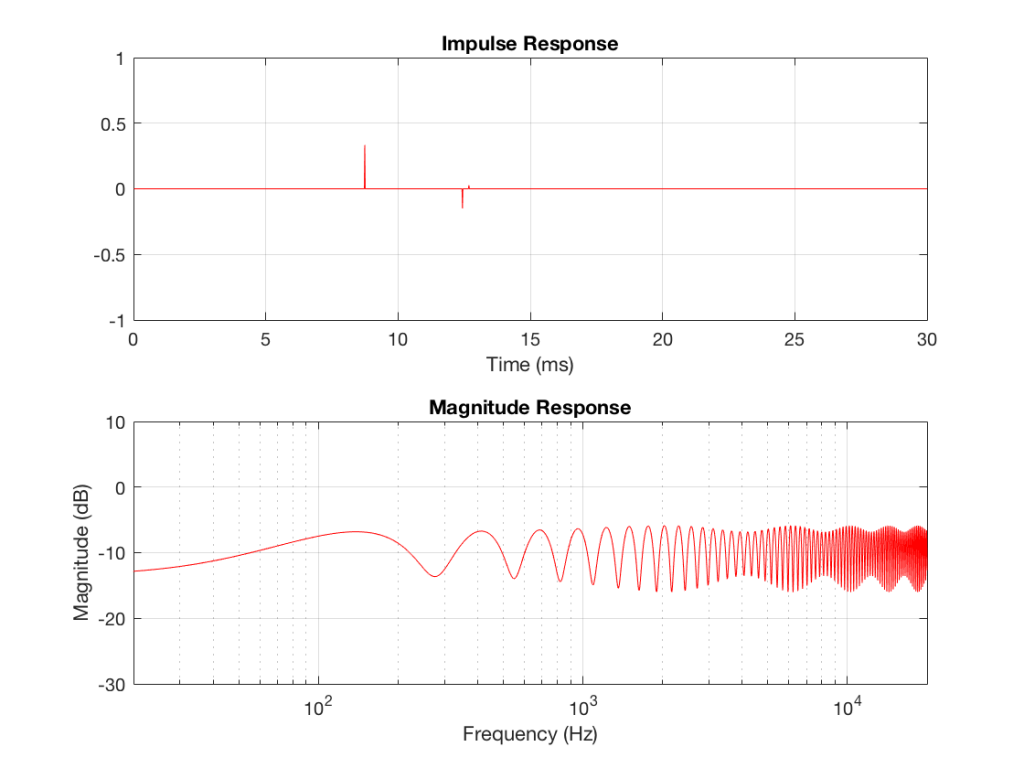
Let’s use the image model to do a very basic prediction of what will happen to our impulse and magnitude responses if we have a single reflection from the left-hand wall.
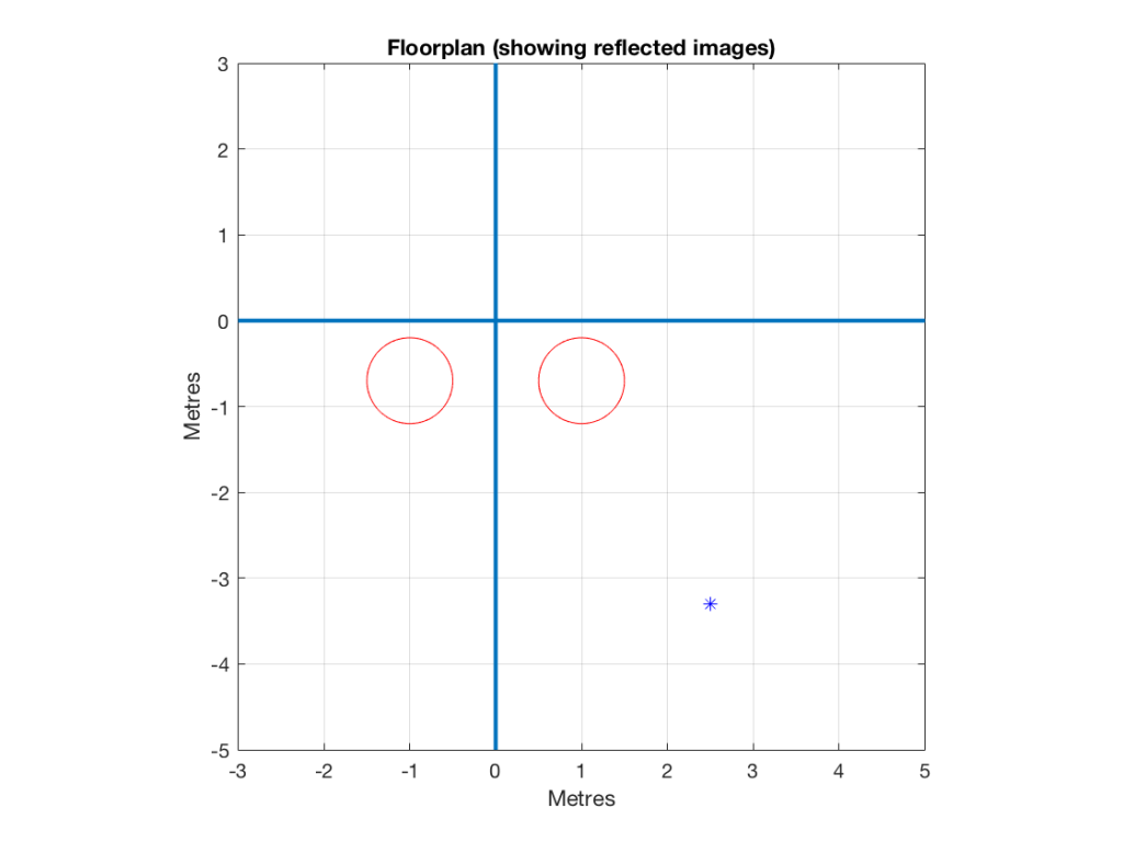

As can be seen in Figure 5, the resulting magnitude response of an omnidirectional loudspeaker with a single, perfect reflection certainly has some noticeable artefacts. If the listening position were closer to the loudspeaker, the artefacts would be smaller, since the reflected signal would be quieter than the direct sound The further away you get, the more the two path lengths are the same, and therefore the bigger the effect on the summed signal.
Of course, this is an unrealistic simulation, since everything is “perfect” – perfect reflection, perfectly omnidirectional loudspeaker with a perfectly flat magnitude response, and so on… However, for the purposes of this posting, that’s good enough.
Let’s now change the directivity of the loudspeaker to alter the balance of level between the direct and the reflected sounds. We’ll make the loudspeaker’s beam width more narrow, giving it the same behaviour as a cardioid microphone (which is called a cardioid because a polar plot of its directivity pattern looks like a heart – cardiovascular and cardioid have the same root).
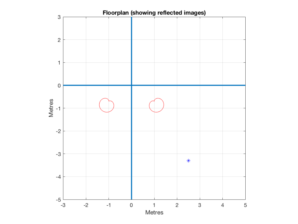

If you look at Figure 7, you’ll see that the times of arrival of the two signals have not changed, but that the effect of the artefact in the frequency domain is reduced (the peaks and dips are smaller). The frequencies of the peaks and dips are the same as in Figure 5 because those are determined by the delay difference between the two spikes in the impulse response. The peaks and dips are smaller because the reflected sound is quieter (because the image loudspeaker – the reflected signal is beaming in a different direction).
Let’s try a different directivity pattern – a dipole, which has a polar patter than looks like a figure “8”.


Notice now that, because the listening position is almost perfectly in line with the “null” – the “dead zone” of the reflected loudspeaker, there is almost nothing to reflect. Consequently, there is very little effect on the on-axis magnitude response of the loudspeaker, as can be seen in the magnitude response in Figure 9.
So, the moral of the story so far is that without moving the loudspeaker or the listening position, or changing the wall’s characteristics, the time response and magnitude response of the loudspeaker at the listening position is heavily dependent on the loudspeaker’s directivity.
Two reflections
Let’s continue the experiment, making the front wall reflective as well.
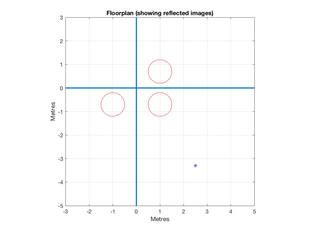

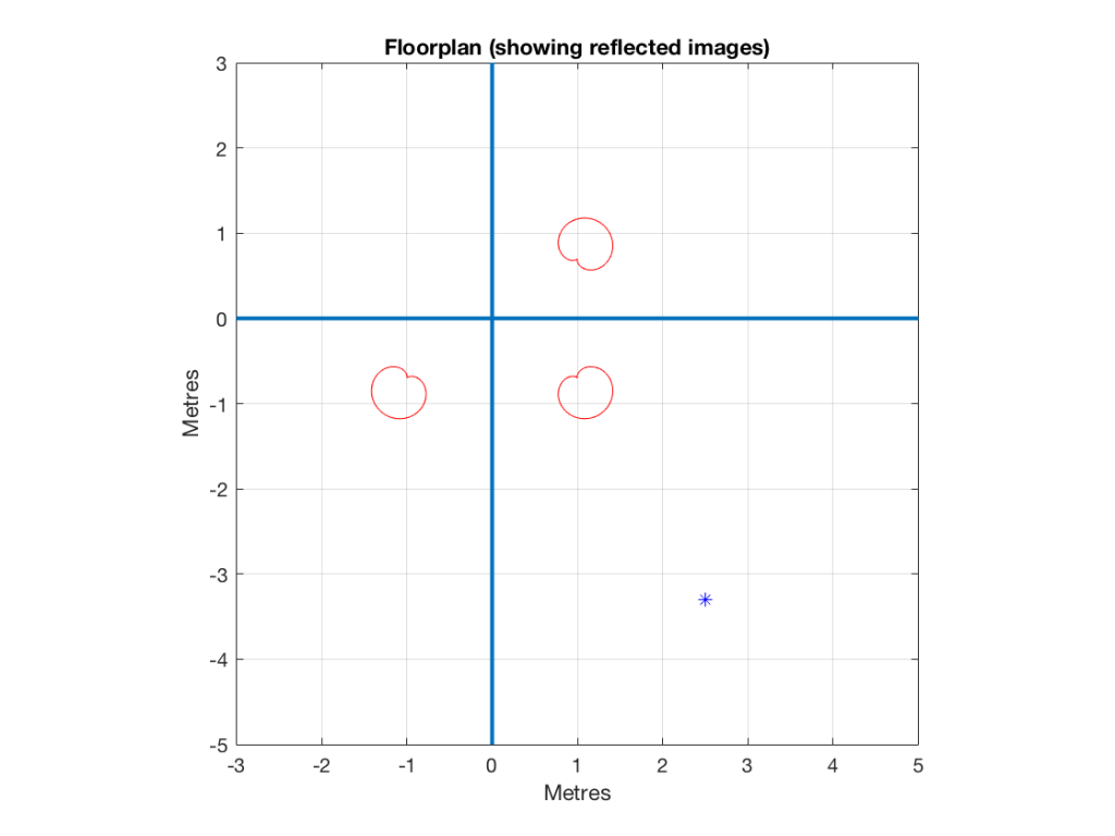


In Figure 15, one additional effect can be seen. Since the reflection off the front wall is negative (in other words, it “pulls” when the direct sound “pushes”) due to the behaviour of the dipole, there is a cancellation in the low frequencies, causing a drop in level in the low end. If we were to push the loudspeaker closer to the front wall, this effect would become more and more obvious.
The moral of the story is…
Of course, this is all very theoretical, however, it should give you an idea of three things.
The first is a simple method of thinking about reflections. You can use the Image Model method to imagine that your walls are mirrors, and you can “see” the other loudspeakers on the other sides of those mirrors. Those images are where your reflections are coming from.
The second is the obvious point – that the summed magnitude response of a loudspeaker’s direct sound, and its reflections is dependent on many things, the directivity being one of them.
The third is possibly the most important. All three of the loudspeaker models I’ve used here have razor-flat on-axis responses in a free field. So, if you were trying to decide which of these three loudspeakers to buy, you’d look at their “frequency response” plots or data and see that all of them are flat to within 0.0001 dB from 1 Hz to infinity Hz, and you’d think that they’d all sound “the same” under the same conditions. However, nothing could be further from the truth. These three loudspeaker with identical on-axis responses will sound completely different. This does not mean that an on-axis magnitude response is useless. It only means that it’s useless in the absence of other information such as the loudspeaker’s power response or its frequency-dependent directivity.
To keep things simple, I have not included frequency-dependent directivity effects. I may do that some day – but beware that it is not enough to say “the loudspeaker beams at higher frequencies so I don’t have to worry about it up there” because that’s not necessarily true – it’s different from loudspeaker to loudspeaker.
This also means that none of the plots I’ve shown here can be used to conclude anything about the real world. All it’s good for is to get a conceptual, intuitive idea of what’s going on when you put a loudspeaker near a wall.
One final comment: the microphone that I’m simulating here has an omnidirectional characteristic. This means that it is as sensitive to the reflected sound as it is to the direct sound, since the angle of incidence of the sound is irrelevant. The way we humans perceive sound is different. We do not perceive the comb filter that the microphone sees when the reflection is coming in from our side, since this is information that is recognised by the brain as being reflected – and it’s used to determine the distance to the sound source. However, if you plug one ear, you may notice that things sound more like you see in the plots, since you lose part of your ability to localise the direction of the signals in the horizontal plane.
For more reading…
Allen, J.B., & Berkley, D.A. (1979) “Image Method for Efficiently Simulating Small-Room Acoustics,” Journal of the Acoustical Society of America, 65(4): 943-950, April.
Eyring, C.F. (1930) “Reverberation Time in ‘Dead’ Rooms,” Journal of the Acoustical Society of America, 1: 217-241.
Gibbs, B.M., & Jones, D.K., (1972) “A Simple Image Method for Calculating the Distribution of Sound Pressure Levels Within an Enclosure,” Acustica, 26: 24-32.