In the April, 1968 issue of Wireless World, there is a short article titled “P.C.M. Copes with Everything”
It’s interesting reading the 57-year old predictions in here. One has proven to be not-quite-correct:
While 27 levels are quite adequate for telephonic speech, 211 or 212 need to be used for high quality music.
I doubt that anyone today would be convinced that 11- or 12-bit PCM would deserve the classification of “high quality”. Although some of my earliest digital recordings were made on a Sony PCM 2500 DAT machine, with an ADC that was only reliable down to about 12 or 13 bits, I wouldn’t try to pass those off as “high quality” recordings.
But, towards the end of the article, it says:
The closing talk was given by A. H. Reeves, the inventor of p.c.m. Letting his imagination take over, he spoke of a world in the not too distant future where communication links will permit people to carry out many jobs from the comfort of their homes, conferences using closed-circuit television etc. For this, he said, reliable links capable of bit rates of the order of 109 or 1010 bits will be required. Light is the most probable answer.
Impressive that, in 1968, Reeves predicted fibre optic connections to our houses and the ability to sit at home on Teams meetings (or Facetime or Zoom or Skype, or whatever…)
I had a little time at work today waiting for some visitors to show up and, as I sometimes do, I pulled an old audio book off the shelf and browsed through it. As usually happens when I do this, something interesting caught my eye.
I was reading the AES publication called “The Phonograph and Sound Recording After One-Hundred Years” which was the centennial issue of the Journal of the AES from October / November 1977.
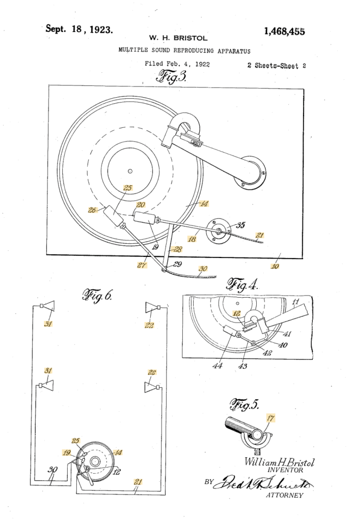
In that issue of the JAES, there is an article called “Record Changers, Turntables, and Tone Arms – A Brief Technical History” by James H. Kogen of Shure Brothers Incorporated, and in that article he mentions US Patent Number 1,468,455 by William H. Bristol of Waterbury, CT, titled “Multiple Sound-Reproducing Apparatus”.
Before I go any further, let’s put the date of this patent in perspective. In 1923, record players existed, but they were wound by hand and ran on clockwork-driven mechanisms. The steel needle was mechanically connected to a diaphragm at the bottom of a horn. There were no electrical parts, since lots of people still didn’t even have electrical wiring in their homes: radios were battery-powered. Yes, electrically-driven loudspeakers existed, but they weren’t something you’d find just anywhere…
In addition, 3- or 2-channel stereo wasn’t invented yet, Blumlein wouldn’t patent a method for encoding two channels on a record until 1931: 8 years in the future…
But, if we look at Bristol’s patent, we see a couple of astonishing things, in my opinion.
If you look at the top figure, you can see the record, sitting on the gramophone (I will not call it a record player or a turntable…). The needle and diaphragm are connected to the base of the horn (seen on the top right of Figure 3, looking very much like my old Telefunken Lido, shown below.
But, below that, on the bottom of Figure 3 are what looks a modern-ish looking tonearm (item number 18) with a second tonearm connected to it (item number 27). Bristol mentions the pickups on these as “electrical transmitters”: this was “bleeding edge” emerging technology at the time.
So, why two pickups? First a little side-story.
Anyone who works with audio upmixers knows that one of the “tricks” that are used is to derive some signal from the incoming playback, delay it, and then send the result to the rear or “surround” loudspeakers. This is a method that has been around for decades, and is very easy to implement these days, since delaying audio in a digital system is just a matter of putting the signal into a memory and playing it out a little later.
Now look at those two tonearms and their pickups. As the record turns, pickup number 20 in Figure 3 will play the signal first, and then, a little later, the same signal will be played by pickup number 26.
Then if you look at Figure 6, you can see that the first signal gets sent to two loudspeakers on the right of the figure (items number 22) and the second signal gets sent to the “surround” loudspeakers on the left (items number 31).
So, here we have an example of a system that was upmixing a surround playback even before 2-channel stereo was invented.
Mind blown…
NB. If you look at Figure 4, you can see that he thought of making the system compatible with the original needle in the horn. This is more obvious in Figures 1 and 2, shown below.
One of the things I have to do occasionally is to test a system or device to make sure that the audio signal that’s sent into it comes out unchanged. Of course, this is only one test on one dimension, but, if the thing you’re testing screws up the signal on this test, then there’s no point in digging into other things before it’s fixed.
One simple way to do this is to send a signal via a digital connection like S/PDIF through the DUT, then compare its output to the signal you sent, as is shown in the simple block diagram in Figure 1.
Figure 1: Basic block diagram of a Device Under Test
If the signal that comes back from the DUT is identical to the signal that was sent to it, then you can subtract one from the other and get a string of 0s. Of course, it takes some time to send the signal out and get it back, so you need to delay your reference signal to time-align them to make this trick work.
The problem is that, if you ONLY do what I described above (using something like the patcher shown in Figure 2) then it almost certainly won’t work.
Figure 2: The wrong way to do it
The question is: “why won’t this work?” and the answer has very much to do with Parts 1 through 4 of this series of postings.
Looking at the left side of the patcher, I’m creating a signal (in this case, it’s pink noise, but it could be anything) and sending it out the S/PDIF output of a sound card by connecting it to a DAC object. That signal connection is a floating point value with a range of ±1.0, and I have no idea how it’s being quantised to the (probably) 24 bits of quantisation levels at the sound card’s output.
That quantised signal is sent to the DUT, and then it comes back into a digital input through an ADC object.
Remember that the signal connection from the pink noise output across to the latency matching DELAY object is a floating point signal, but the signal coming into the ADC object has been converted to a fixed point signal and then back to a floating point representation.
Therefore, when you hit the subtraction object, you’re subtracting a floating point signal from what is effectively a fixed point quantised signal that is coming back in from the sound card’s S/PDIF input. Yes, the fixed point signal is converted to floating point by the time it comes out of the ADC object – but the two values will not be the same – even if you just connect the sound card’s S/PDIF output to its own input without an extra device out there.
In order to give this test method a hope of actually working, you have to do the quantisation yourself. This will ensure that the values that you’re sending out the S/PDIF output can be expected to match the ones you’re comparing them to internally. This is shown in Figure 3, below.
Figure 3: A better way to do it
Notice now that the original floating point signal is upscaled, quantised, and then downscaled before its output to the sound card or routed over to the comparison in the analysis section on the right. This all happens in a floating point world, but when you do the rounding (the quantisation) you force the floating point value to the one you expect when it gets converted to a fixed point signal.
This ensures that the (floating point) values that you’re using as your reference internally CAN match the ones that are going through your S/PDIF connection.
In this example, I’ve set the bit depth to 16 bits, but I could, of course, change that to whatever I want. Typically I do this at the 24-bit level, since the S/PDIF signal supports up to 24 bits for each sample value.
Be careful here. For starters, this is a VERY basic test and just the beginning of a long series of things to check. In addition, some sound cards do internal processing (like gain or sampling rate conversion) that will make this test fail, even if you’re just doing a loop back from the card’s S/PDIF output to its own input. So, don’t copy-and-paste this patcher and just expect things to work. They might not.
But the patcher shown in Figure 2 definitely won’t work…
One small last thing
You may be wondering why I take the original signal and send it to the right side of the “-” object instead of making things look nice by putting it in the left side. This is because I always subtract my reference signal from the test signal and not the other way around. Doing this every time means that I don’t have to interpret things differently every time, trying to figure out whether things are right-side-up or upside-down.
It is often the case that you have to convert a floating point representation to a fixed point representation. For example, you’re doing some signal processing like changing the volume or adding equalisation, and you want to output the signal to a DAC or a digital output.
The easiest way to do this is to just send the floating point signal into the DAC or the S/PDIF transmitter and let it look after things. However, in my experience, you can’t always trust this. (I’ll explain why in a later posting in this series.) So, if you’re a geek like me, then you do this conversion yourself in advance to ensure you’re getting what you think you’re getting.
To start, we’ll assume that, in the floating point world, you have ensured that your signal is scaled in level to have a maximum amplitude of ± 1.0. In floating point, it’s possible to go much higher than this, and there’re no serious reason to worry going much lower (see this posting). However, we work with the assumption that we’re around that level.
So, if you have a 0 dB FS sine wave in floating point, then its maximum and minimum will hit ±1.0.
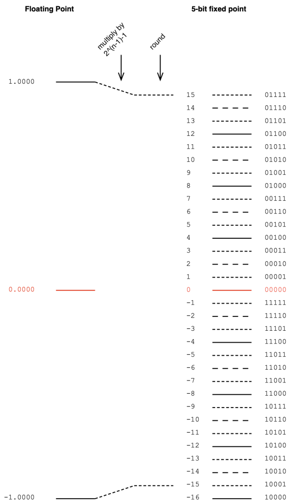
Then, we have to convert that signal with a range of ±1.0 to a fixed point system that, as we already know, is asymmetrical. This means that we have to be a little careful about how we scale the signal to avoid clipping on the positive side. We do this by multiplying the ±1.0 signal by 2^(nBits-1)-1 if the signal is not dithered. (Pay heed to that “-1” at the end of the multiplier.)
Let’s do an example of this, using a 5-bit output to keep things on a human scale. We take the floating point values and multiply each of them by 2^(5-1)-1 (or 15). We then round the signals to the nearest integer value and save this as a two’s complement binary value. This is shown below in Figure 1.
Figure 1. Converting floating point to a 5-bit fixed point value without dither.
As should be obvious from Figure 1, we will never hit the bottom-most fixed point quantisation level (unless the signal is asymmetrical and actually goes a little below -1.0).
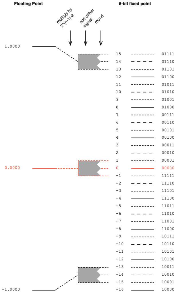
If you choose to dither your audio signal, then you’re adding a white noise signal with an amplitude of ±1 quantisation level after the floating point signal is scaled and before it’s rounded. This means that you need one extra quantisation level of headroom to avoid clipping as a result of having added the dither. Therefore, you have to multiply the floating point value by 2^(nBits-1)-2 instead (notice the “-2” at the end there…) This is shown below in Figure 2.
Figure 2. Converting floating point to a 5-bit fixed point value with dither.
Of course, you can choose to not dither the signal. Dither was a really useful thing back in the days when we only had 16 reliable bits to work with. However, now that 24-bit signals are normal, dither is not really a concern.
In Part 1 of this series, I talked about three different options for converting from a fixed-point representation to another fixed-point representation with a bigger bit depth.
This happens occasionally. The simplest case is when you send a 16-bit signal to a 24-bit DAC. Another good example is when you send a 16-bit LPCM signal to a 24- or 32-bit fixed point digital signal processor.
However, these days it’s more likely that the incoming fixed-point signal (incoming signals are almost always in a fixed-point representation) is converted to floating point for signal processing. (I covered the differences between fixed- and floating-point representations in another posting.)
If you’re converting from fixed point to floating point, you divide the sample’s value by 2^(nBits-1). In other words, if you’re converting a 5-bit signal to floating point, you divide each sample’s value by 2^4, as shown below.
Figure 1. Converting a 5-bit fixed point signal to floating point
The reason for this is that there are 2^(nBits-1) quantisation levels for the negative portions of the signal. The positive-going portions have one fewer levels due to the two’s complement representation (the 00000 had to come from somewhere…).
So, you want the most-negative value to correspond to -1.0000 in the floating point world, and then everything else looks after itself.
Of course, this means that you will never hit +1.0. You’ll have a maximum signal level of 1 – 1/2^(nBits-1), which is very close. Close enough.
The nice thing about doing this conversation is that by entering into a floating point world, you immediately gain resolution to attenuate and headroom to increase the gain of the signal – which is exactly what we do when we start processing things.
Of course, this also means that, when you’re done processing, you’ll need to feed the signal out to a fixed-point world again (for example, to a DAC or to an S/PDIF output). That conversion is the topic of Part 4.
This is the first of a series of postings about strategies for converting from one bit depth to another, including conversion back and forth between fixed point and floating point encoding. It’ll be focusing on a purely practical perspective, with examples of why you need to worry about these things when you’re doing something like testing audio devices or transmission systems.
As we go through this, it might be necessary to do a little review, which means going back and reading some other postings I’ve done in the past if some of the concepts are new. I’ll link back to these as we need them, rather than hitting you with them all at once.
To start, if you’re not familiar with the concept of quantisation and bit depth in an LPCM audio signal, I suggest that you read this posting.
Now that you’re back, you know that if you’re just converting a continuous audio signal to a quantised LPCM version of it, the number of bits in the encoded sample values can be thought of as a measure of the system’s resolution. The more bits you have, the more quantisation steps, and therefore the better the signal to noise ratio.
However, this assumes that you’re using as many of the quantisation steps as possible – in other words, it assumes that you have aligned levels so that the highest point in the audio signal hits the highest possible quantisation step. If your audio signal is 6 dB lower than this, then you’re only using half of your available quantisation values. In other words, if you have a 16-bit ADC, and your audio signal has a maximum peak of -6 dB FS Peak, then you’ve done a 15-bit recording.
But let’s say that you already have an LPCM signal, and you want to convert it to a larger bit depth. A very normal real-world example of this is that you have a 16-bit signal that you’ve ripped from a CD, and you export it as a 24-bit wave file. Where do those 8 extra bits come from and where do they go?
Generally speaking, you have 3 options when you do this “conversion”, and the first option I’ll describe below is, by far the most common method.
Option 1: Zero padding
Let’s simplify the bit depths down to human-readable sizes. We’ll convert a 3-bit LPCM audio signal (therefore it has 2^3 = 8 quantisation steps) into a 5-bit representation (2^5 = 32 quantisation steps), instead of 16-bit to 24-bit. That way, I don’t have to type as many numbers into my drawings. The basic concepts are identical, I’ll just need fewer digits in this version.
The simplest method to do is to throw some extra zeros on the right side of our original values, and save them in the new format. A graphic version of this is shown in Figure 1.
Figure 1. Zero-padding to convert to a higher bit depth.
There are a number of reasons why this is a smart method to use (which also explains why this is the most common method).
The first is that there is no change in signal level. If you have a 0 dB FS Peak signal in the 3-bit world, then we assume that it hits the most-negative value of 100. If you zero-pad this, then the value becomes 10000, which is also the most-negative value in the 5-bit world. If you’re testing with symmetrical signals (like a sinusoidal tone) then you never hit the most-negative value, since this would mean that it would clip on the positive side. This might result in a test that’s worth talking about, since sinusoidal tone that hits 011 and is then converted to 01100. In the 5-bit world, you could make a tone that is a little higher in level (by 3 quantisation levels – those top three dotted lines on the right side of Figure 1), but that difference is very small in real life, so we ignore it. The biggest reason for ignoring this is that this extra “headroom” that you gain is actually fictitious – it’s an artefact of the fact that you typically test signal levels like this with sine tones, which are symmetrical.
The second reason is that this method gives you extra resolution to attenuate the signal. For example, if you wanted to make a volume knob that only attenuated the audio signal, then this conversion method is a good way to do it. (For example, you send a 16-bit digital signal into the input of a loudspeaker with a volume controller. You zero-pad the signal to 24-bit and you now have the ability to reduce the signal level by 141 dB instead of just 93 dB (assuming that you’re using dither…). This is good if the analogue dynamic range of the rest of the system “downstream” is more than 93 dB.) The extra resolution you get is equivalent to 6 dB * each extra bit. So, in the system above:
(5 bits – 3 bits) = 2 extra bits 2 extra bits * 6 dB = 12 dB extra resolution
There is one thing to remember when doing it this way, that you may consider to be a disadvantage. This is the fact that you can’t increase the gain without clipping. So, let’s say that you’re building a digital equaliser or a mixer in a fixed-point system, then you can’t just zero-pad the incoming signal and think that you can boost signals or add them. If you do this, you’ll clip. So, you would have to zero-pad at the input, then attenuate the signal to “buy” yourself enough headroom to increase it again with the EQ or by mixing.
Option 2
The second option is, in essence, the same as the trick I just explained in the previous paragraph. With this method, you don’t ONLY pad the right side of the values with zeros, you pad the values on the left as well with either a 1 or a 0, depending on whether the signals are positive or negative. This means that your “old” value is inserted into the middle of the new value, as shown below in Figure 2. (In this 3- to 5-bit example, this is identical to using option 1, and then dropping the signal level by 6 dB (1 of the 2 bits)).
If your conversion to the bigger bit depth is done inside a system where you know what you’ve done, and if you need room to scale the level of the signal up and down, this is a clever and simple way to do things. There are some systems that did this in the past, but since it’s a process that’s done internally, and we normal people sit outside the system, there’s no real way for us to know that they did it this way.
(For example, I once heard through the grapevine that there was a DAW that imported 24-bits into a 48-bit fixed point processing system, where they padded the incoming files with 12 bits on either side to give room to drop levels on the faders and also be able to mix a lot of full-scale signals without clipping the output.)
Option 3
I only add the third option as a point of completion. This is an unusual way to do a conversion, and I only personally know of one instance where it’s been used. This only means that it’s not a common way to do things – not that NO ONE does it.
In this method, all the padding is done on the left side of the binary values, as shown below in Figure 3.
If we’re thinking along the same lines as in Options 1 and 2, then you could say that this system does not add resolution to attenuate signals, but it does give you the option to make them louder.
However, as we’ll see in Part 2 of this series, there is another advantage to doing it this way…
Nota Bene
I’ve written everything above this line, intentionally avoiding a couple of common terms, but we’ll need those terms in our vocabulary before moving on to Part 2.
If you look at the figures above, and start at the red 0 line, as you go upwards, the increase in signal can be seen as an increase in the left-most bits in each quantisation value. Reading from left-to-right, the first bit tells us whether the value is positive (0) or negative (1), but after this (for the positive values) the more 1s you have on the left, the higher the level. This is why we call them the Most Significant Bits or MSBs. Of course, this means that the last bit on the right is the Least Significant Bit or LSB.
This means that I could have explained Option 1 above by saying:
The three bits of the original signal become the three MSBs of the new signal.
… which also tells us that the signal level will not drop when converted to the 5-bit system.
Or I could have explained Option 3 by saying:
The three bits of the original signal become the three LSBs of the new signal.
.. which also tells us that the signal level will drop when converted to the 5-bit system.
Being able to think in terms of LSBs and MSBs will be helpful later.
Finally… yes, we will talk about Floating Point representations. Later. But if you can’t wait, read this in the meantime.
After I posted the last two parts of this series (which I thought wrapped it up…) I received an email asking about whether there’s a similar thing happening if you remove the reconstruction (low-pass) filter in the digital-to-analogue part of the signal path.
The answer to this question turned out to be more interesting than I expected… So I wound up turning it into a “Part 3” in the series.
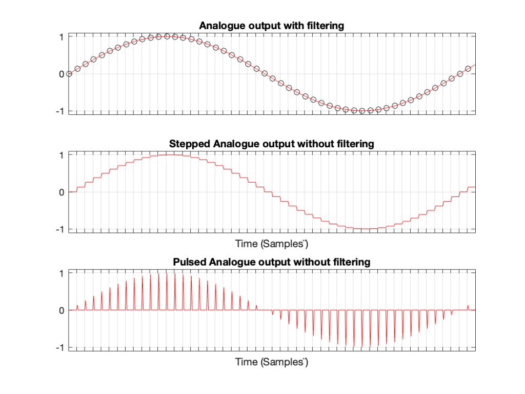
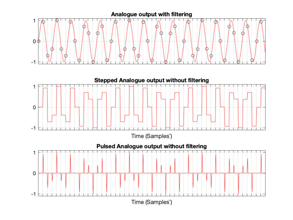
Let’s take a case where you have a 1 kHz signal in a 48 kHz system. The figure below shows three plots. The top plot shows the individual sample values as black circles on a red line, which is the analogue output of a DAC with a reconstruction filter.
The middle plot shows what the analogue output of the DAC would look like if we implemented a Sample-and-hold on the sample values, and we had an infinite analogue bandwidth (which means that the steps have instantaneous transitions and perfect right angles).
The bottom plot shows what the analogue output of the DAC would look like if we implemented the signal as a pulse wave instead, but if we still we had an infinite analogue bandwidth. (Well… sort of…. Those pulses aren’t infinitely short. But they’re short enough to continue with this story.)
Figure 1. A 1 kHz sine wave
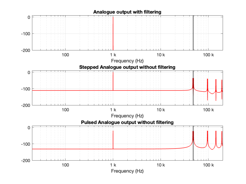
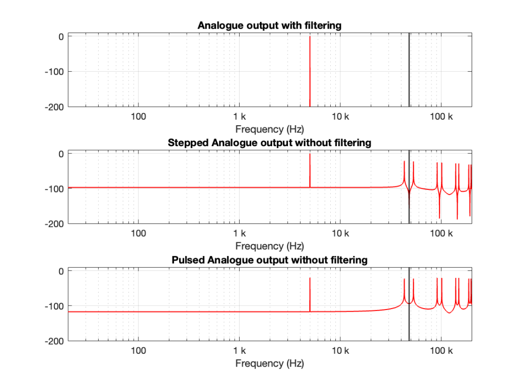
If we calculate the spectra of these three signals , they’ll look like the responses shown in Figure 2.
Figure 2. The spectra of the signals in Figure 1.
Notice that all three have a spike at 1 kHz, as we would expect. The outputs of the stepped wave and the pulsed wave have much higher “noise” floors, as well as artefacts in the high frequencies. I’ve indicated the sampling rate at 48 kHz as a vertical black line to make things easy to see.
We’ll come back to those artefacts below.
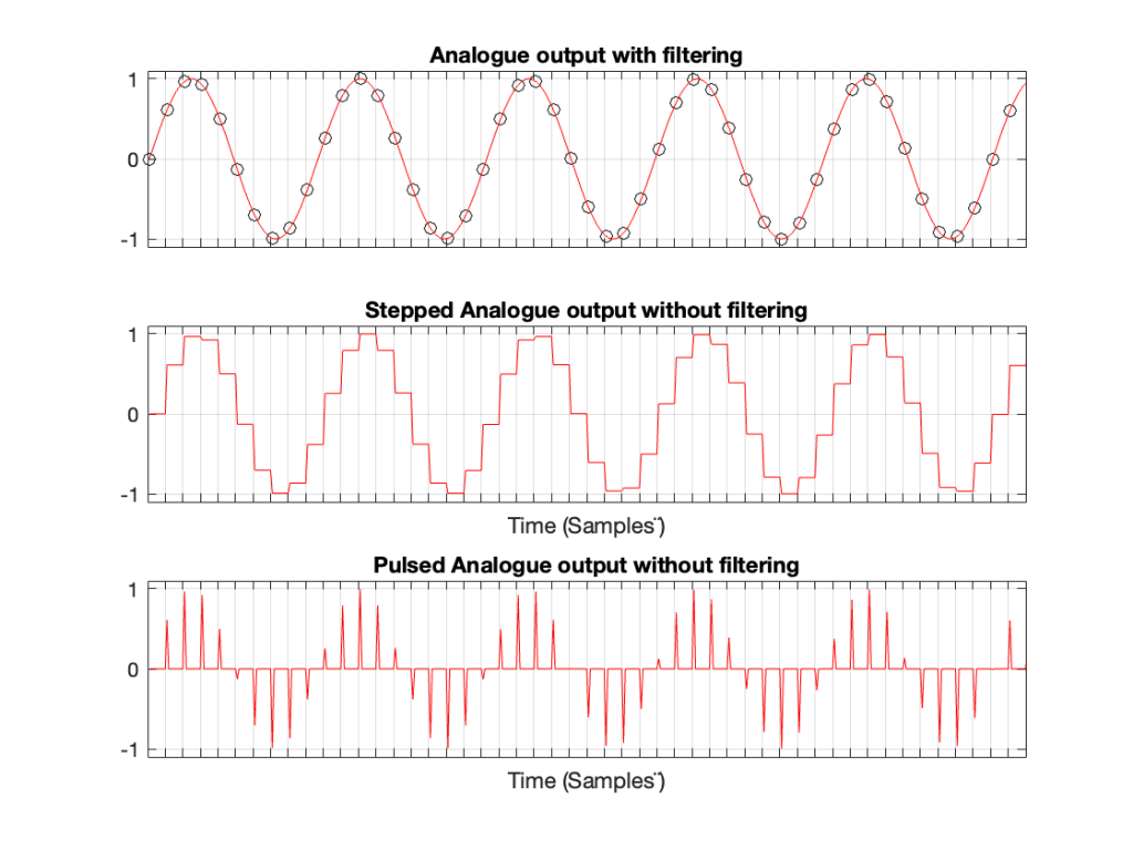
Let’s do the same thing for a 5 kHz sine wave, still in a 48 kHz system, seen in Figures 3 and 4.
Figure 3. A 5 kHz sine wave
Figure 4. The spectra of the signals in Figure 3.
Compare the high-frequency artefacts in Figure 4 to those in Figure 2.
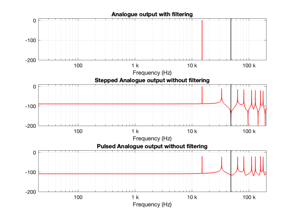
Now, we’ll do it again for a 15 kHz sine wave.
Figure 5. A 15 kHz sine wave
Figure 6. The spectra of the signals in Figure 5.
There are three things to notice, comparing Figures 2, 4, and 6.
The first thing is that artefacts for the stepped and pulsed waves have the same frequency components.
The second thing is that those artefacts are related to the signal frequency and the sampling rate. For example, the two spikes immediately adjacent to the sampling rate are Fs ± Fc where Fs is the sampling rate and Fc is the frequency of the sine wave. The higher-frequency artefacts are mirrors around multiples of the sampling rate. So, we can generalise to say that the artefacts will appear at
n * Fs ± Fc
where n is an integer value.
This is interesting because it’s aliasing, but it’s aliasing around the sampling rate instead of the Nyquist Frequency, which is what happens at the ADC and inside the digital domain before the DAC.
The third thing is a minor issue. This is the fact that the level of the fundamental frequency in the pulsed wave is lower than it is for the stepped wave. This should not be a surprise, since there’s inherently less energy in that wave (since, most of the time, it’s sitting at 0). However, the artefacts have roughly the same levels; the higher-frequency ones have even higher levels than in the case of the stepped wave. So, the “signal to THD+N” of the pulsed wave is lower than for the stepped wave.
In Part 1, we looked at what happens when you try to record a signal whose frequency is higher than 1/2 the sampling rate (which, from now on, I’ll call the Nyquist Frequency, named after Harry Nyquist who was one of the people that first realised that this limit existed). You record a signal, but it winds up having a different frequency at the output than it had at the input. In addition, that frequency is related to the signal’s frequency and the sampling rate itself.
In order to prevent this from happening, digital recording systems use a low-pass filter that hypothetically prevents any signals above the Nyquist frequency from getting into the analogue-to-digital conversion process. This filter is called an anti-aliasing filter because it prevents any signals that would produce an alias frequency from getting into the system. (In practice, these filters aren’t perfect, and so it’s typical that some energy above the Nyquist frequency leaks into the converter.)
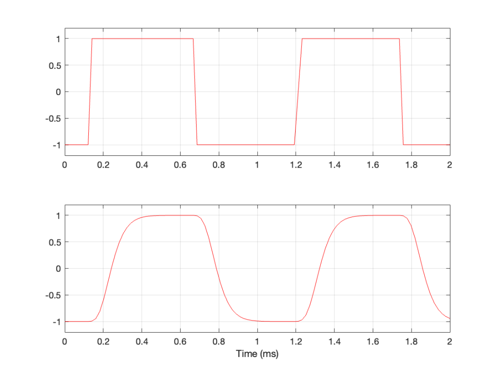
So, this means that if you put a signal that contains high frequency components into the analogue input of an analogue-to-digital converter (or ADC), it will be filtered. An example of this is shown in Figure 1, below. The top plot is a square wave before filtering. The bottom plot is the result of low-pass filtering the square wave, thus heavily attenuating its higher harmonics. This results in a reduction in the slope when the wave transitions between low and high states.
Figure 1: A square wave before and after low-pass filtering.
This means that, if I have an analogue square wave and I record it digitally, the signal that I actually record will be something like the bottom plot rather than the top one, depending on many things like the frequency of the square wave, the characteristics of the anti-aliasing filter, the sampling rate, and so on. Don’t go jumping to conclusions here. The plot above uses an aggressively exaggerated filter to make it obvious that we do something to prevent aliasing in the recorded signal. Do NOT use the plots as proof that “analogue is better than digital” because that’s a one-dimensional and therefore very silly thing to claim.
However…
… just because we keep signals with frequency content above the Nyquist frequency out of the input of the system doesn’t mean that they can’t exist inside the system. In other words, it’s possible to create a signal that produces aliasing after the ADC. You can either do this by
creating signals from scratch (for example, generating a sine tone with a frequency above Nyquist) or
by producing artefacts because of some processing applied to the signal (like clipping, for example).
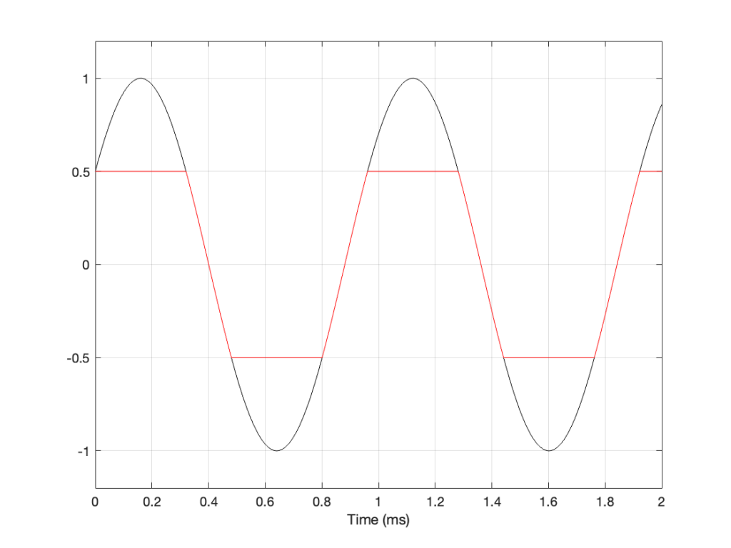
Let’s take a sine wave and clip it after it’s been converted to a digital signal with a 48 kHz sampling rate, as is shown in Figure 2.
Figure 2: The red curve is a clipped version of the black curve.
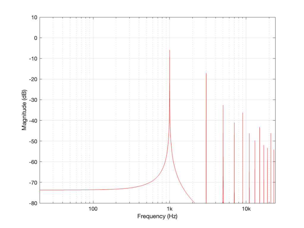
When we clip a signal, we generate high-frequency harmonics. For example, the signal in Figure 2 is a 1 kHz sine wave that I clipped at ±0.5. If I analyse the magnitude response of that, it will look something like Figure 3:
Figure 3: The magnitude response of Figure 2, showing the upper harmonics that I created by clipping.
The red curve in Figure 2 is not a ‘perfect’ square wave, so the harmonics seen in Figure 3 won’t follow the pattern that you would expect for such a thing. But that’s not the only reason this plot will be weird…
Figure 3 is actually hiding something from you… I clipped a 1 kHz sine wave, which makes it square-ish. This means that I’ve generated harmonics at 3 kHz, 5 kHz, 7 kHz, and so on, up to ∞ Hz..
Notice there that I didn’t say “up to the Nyquist frequency”, which, in this example with a sampling rate of 48 kHz, would be 24 kHz.
Those harmonics above the Nyquist frequency were generated, but then stored as their aliases. So, although there’s a new harmonic at 25 kHz, the system records it as being at 48 kHz – 25 kHz = 23 kHz, which is right on top of the harmonic just below it.
In other words, when you look at all the spikes in the graph in Figure 3, you’re actually seeing at least two spikes sitting on top of each other. One of them is the “real” harmonic, and the other is an alias (there are actually more, but we’ll get to that…). However, since I clipped a 1 kHz sine wave in a 48 kHz world, this lines up all the aliases to be sitting on top of the lower harmonics.
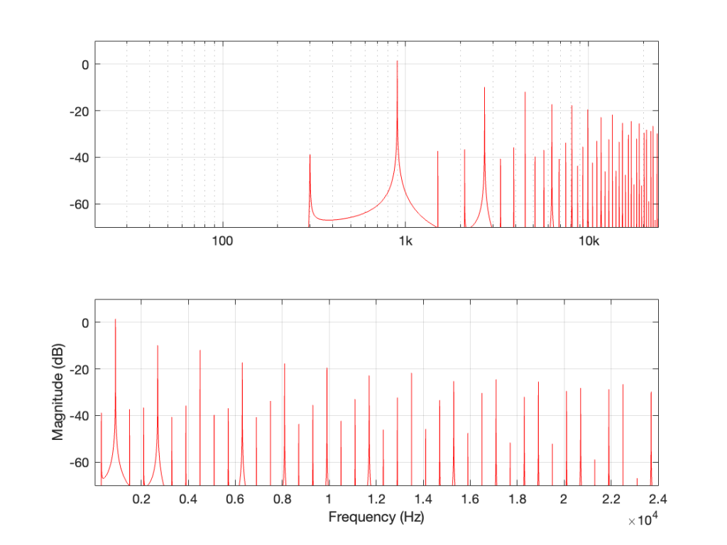
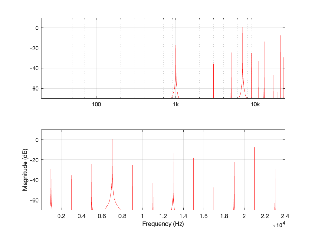
So, what happens if I clip a sine wave with a frequency that isn’t nicely related to the sampling rate, like 900 Hz in a 48 kHz system, for example? Then the result will look more like Figure 4, which is a LOT messier.
Figure 4: The magnitude response of a 900 Hz square wave, plotted with a logarithmic frequency axis in the top axis and a linear axis in the bottom.
A 900 Hz square wave will have harmonics at odd multiples of the fundamental, therefore at 2.7 kHz, 4.5 kHz, and so on up to 22.5 kHz (900 Hz * 25).
The next harmonic is 24.3 kHz (900 Hz * 27), which will show up in the plots at 48 kHz – 24.3 kHz = 23.7 kHz. The next one will be 26.1 kHz (900 Hz * 29) which shows up in the plots at 21.9 kHz. This will continue back DOWN in frequency through the plot until you get to 900 Hz * 53 = 47.7 kHz which will show up as a 300 Hz tone, and now we’re on our way back up again… (Take a look at Figure 7, below for another way to think of this.)
The next harmonic will be 900 Hz * 55 = 49.5 kHz which will show up in the plot as a 1.5 kHz tone (49.5 kHz – 48 kHz).
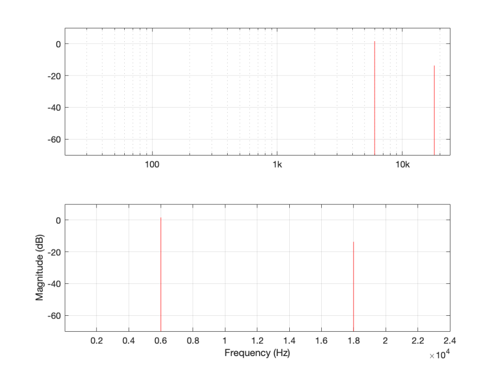
Depending on the relationship between the square wave’s frequency and the sampling rate, you either get a “pretty” plot, like for the 6 kHz square wave in a 48 kHz system, as shown in Figure 5.
Figure 5: the magnitude response of a 6 kHz square wave in a 48 kHz system
Or, it’s messy, like the 7 kHz square wave in a 48 kHz system in Figure 6.
Figure 6: The magnitude response of a 7 kHz square wave in a 48 kHz system.
The moral of the story
There are three things to remember from this little pair of posts:
Some aliased artefacts are negative frequencies, meaning that they appear to be going backwards in time as compared to the original (just like the wheel appearing to rotate backwards in Part 1).
Just because you have an antialiasing filter at the input of your ADC does NOT protect you from aliasing, because it can be generated internally, after the signal has been converted to the digital domain.
Once this aliasing has happened (e.g. because you clipped the signal in the digital domain), then the aliases are in the signal below the Nyquist frequency and therefore will not be removed by the reconstruction low-pass filter in the DAC. Once they’re mixed in there with the signal, you can’t get them out again.
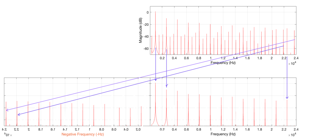
Figure 7: This is the same as Figure 4, but I’ve removed the first set of mirrored alias artefacts and plotted them on the left side as being mirrored in a “negative frequency” alternate universe.
One additional, but smaller problem with all of this is that, when you look at the output of an FFT analysis of a signal (like the top plot in Figure 7, for example), there’s no way for you to know which components are “normal” harmonics, and which are aliased artefacts that are actually above the Nyquist frequency. It’s another case proving that you need to understand what to expect from the output of the FFT in order to understand what you’re actually getting.
One of the best-known things about digital audio is the fact that you cannot record a signal that has a frequency that is higher than 1/2 the sampling rate.
Now, to be fair, that statement is not true. You CAN record a signal that has a frequency that is higher than 1/2 the sampling rate. You just won’t be able to play it back properly, because what comes out of the playback will not be the original frequency, but an alias of it.
If you record a one-spoked wheel with a series of photographs (in the old days, we called this ‘a movie’), the photos (the frames of the movie) might look something like this:
As you can see there, the wheel happens to be turning at a speed that results in it rotating 45º every frame.
The equivalent of this in a digital audio world would be if we were recording a sine wave that rotated (yes…. rotated…) 45º every sample, like this:
Notice that the red lines indicating the sample values are equivalent to the height of the spoke at the wheel rim in the first figure.
If we speed up the wheel’s rotation so that it rotated 90º per frame, it looks like this:
And the audio equivalent would look like this:
Speeding up even more to 135º per frame, we get this:
and this:
Then we get to a magical speed where the wheel rotated 180º per frame. At this speed, it appears when we look at the playback of the film that the wheel has stopped, and it now has two spokes.
In the audio equivalent, it looks like the result is that we have no output, as shown below.
However, this isn’t really true. It’s just an artefact of the fact that I chose to plot a sine wave. If I were to change the phase of this to be a cosine wave (at the same frequency) instead, for example, then it would definitely have an output.
At this point, the frequency of the audio signal is 1/2 the sampling rate.
What happens if the wheel goes even faster (and audio signal’s frequency goes above this)?
Notice that the wheel is now making more than a half-turn per frame. We can still record it. However, when we play it back, it doesn’t look like what happened. It looks like the wheel is going backwards like this:
Similarly, if we record a sine wave that has a frequency that is higher than 1/2 the sampling rate like this:
Then, when we play it back, we get a lower frequency that fits the samples, like this:
Just a little math
There is a simple way to calculate the frequency of the signal that you get out of the system if you know the sampling rate and the frequency of the signal that you tried to record.
Let’s use the following abbreviations to make it easy to state:
Fs = Sampling rate
F_in = frequency of the input signal
F_out = frequency of the output signal
IF F_in < Fs/2 THEN F_out = F_in
IF Fs > F_in > Fs/2 THEN F_out = Fs/2 – (F_in – Fs/2) = Fs – F_in
Some examples:
If your sampling rate is 48 kHz, and you try to record a 25 kHz sine wave, then the signal that you will play back will be: 48000 – 25000 = 23000 Hz
If your sampling rate is 48 kHz, and you try to record a 42 kHz sine wave, then the signal that you will play back will be: 48000 – 42000 = 6000 Hz
So, as you can see there, as the input signal’s frequency goes up, the alias frequency of the signal (the one you hear at the output) will go down.
There’s one more thing…
Go back and look at that last figure showing the playback signal of the sine wave. It looks like the sine wave has an inverted polarity compared to the signal that came into the system (notice that it starts on a downwards-slope whereas the input signal started on an upwards-slope). However, the polarity of the sine wave is NOT inverted. Nor has the phase shifted. The sine wave that you’re hearing at the output is going backwards in time compared to the signal at the input, just like the wheel appears to be rotating backwards when it’s actually going forwards.
In Part 2, we’ll talk about why you don’t need to worry about this in the real world, except when you REALLY need to worry about it.