Back to Part 2

Signal Levels

Every audio device relies on a rather simple balancing act. The “signal”, whether it’s speech, music, or sound effects, should be loud enough to mask the noise that is inherent in the recording or transmission itself. The measurement of this “distance” in level is known as the Signal-to-Noise Ratio or SNR. However, the signal should not be so loud as to overload the system and cause distortion effects such as clipping, which results in what is commonly called Total Harmonic Distortion or THD.(1) One basic method to evaluate the quality of an audio signal or device is to group these two measurements into one value: the Total Harmonic Distortion plus Noise or THD+N value. The somewhat challenging issue with this value is that a portion of it (the noise floor) is typically independent of the signal level, since a device or signal will have some noise regardless of whether a signal is present or not. However, the distortion is typically directly related to the level of the signal.

In modern digital PCM audio signal (assuming that it is correctly-implemented and ignoring any additional signal processing), the noise floor is the result of the dither that is used to randomise the inherent quantisation error in the encoding system. This noise is independent of the signal level, and entirely dependent on the resolution of the system (measured in the number of bits used to encode each sample). The maximum possible level that can be encoded without incurring additional distortion that is inherent in the encoding system itself is when the maximum (or minimum) value in the audio signal reaches the highest possible signal value of the system. Any increase in the signal’s level beyond this will be clipped, and harmonic distortion artefacts will result.

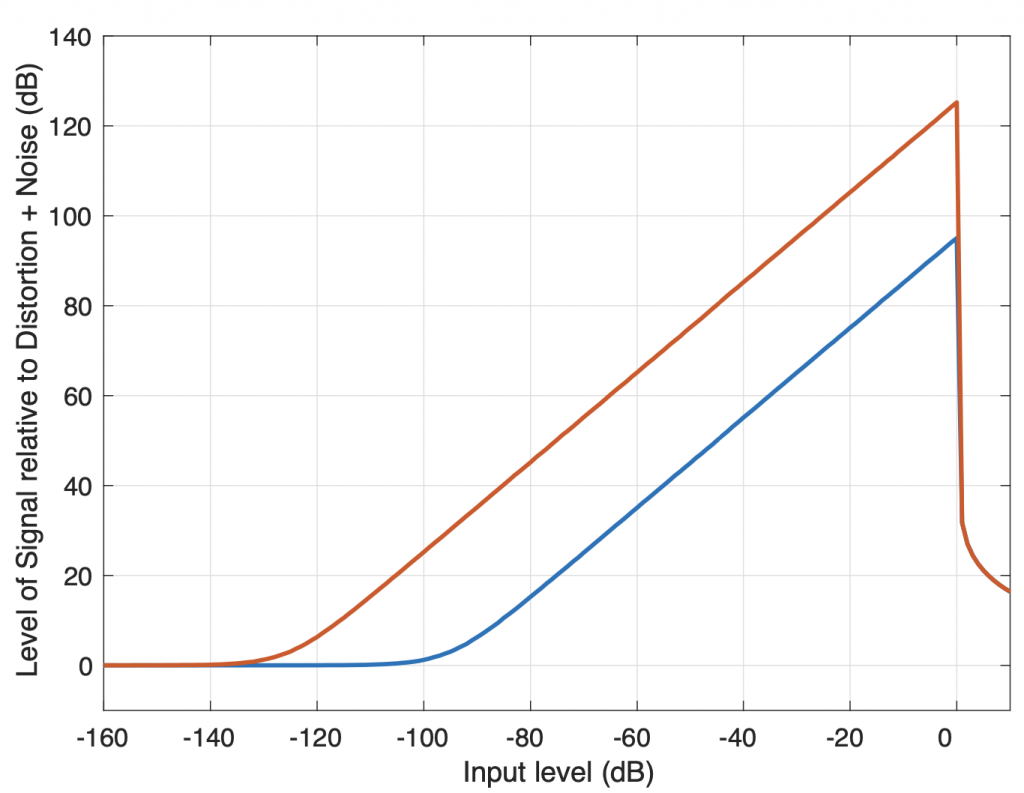
Figure 1 shows two examples of the relationship between the levels of the signal and the THD+N in a digital audio system. The red line shows a 24-bit encoding, the blue line is for 16-bit. The “flat line” on the left of the plot is the result of the noise floor of the system. In this region, the signal level is so low, it’s below the noise floor of the system itself, so the only measurable output is the noise, and not the signal. As we move towards the right, the input signal gets louder and raises above the noise floor, so the output level naturally increases as well. However, in a digital audio system, we reach a maximum possible input level of 0 dB FS. If we try to increase the signal’s level above this, the signal itself will not get louder, however, it will become more and more distorted. As a result, the distortion artefacts quickly become almost as loud as the signal itself, and so the plots drop dramatically.

This is why good recording engineers typically attempt to align the levels of the microphones to ensure that the maximum peak of the entire recording will just barely reach the maximum possible level of the digital recording system. This ensures that they are keeping above the noise floor as much as possible without distorting the signals.

Audio signals recorded on analogue-only devices generally have the same behaviour; there is a noise floor that should be avoided and a maximum level above which distortion will start to increase. However, many analogue systems have a slightly different characteristic, as can be seen in the idealised model shown in Figure 2. Notice that, just like in the digital audio system, the noise floor is constant, and as the level of the input signal is increased, it rises above this. However, in an analogue system, the transition to a distorted signal is more gradual, seen as the more gentle slopes of the curves on the right side of the graph.

As a result, in a typical analogue audio system, there is an “optimal” level that is seen to be the best compromise between the signal being loud enough above the noise floor, but not distorting too much. The question of how much distortion is “too much” can then be debated — or even used as an artistic effect (as in the case of so-called “tape compression”).

If we limit our discussion to the stylus tracking a groove on a vinyl disc, converting that movement to an electrical signal that is amplified and filtered in a RIAA-spec preamplifier, then a phonograph recording is an analogue format. This means, generally speaking, that there is an optimal level for the audio signal, which, in the case of vinyl, means a modulation velocity of the stylus, converted to an electrical voltage.

Although there are some minor differences of opinion, a commonly-accepted optimum level for the groove on a stereo recording is 35.4 mm/sec for a single audio channel at 1,000 Hz. In a case where both audio channels have the same 1 kHz signal recorded in phase (as a dual-monophonic signal), then this means that the lateral velocity of the stylus will be 50 mm/sec.(2)

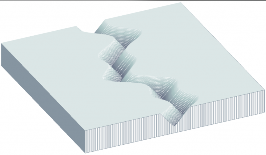
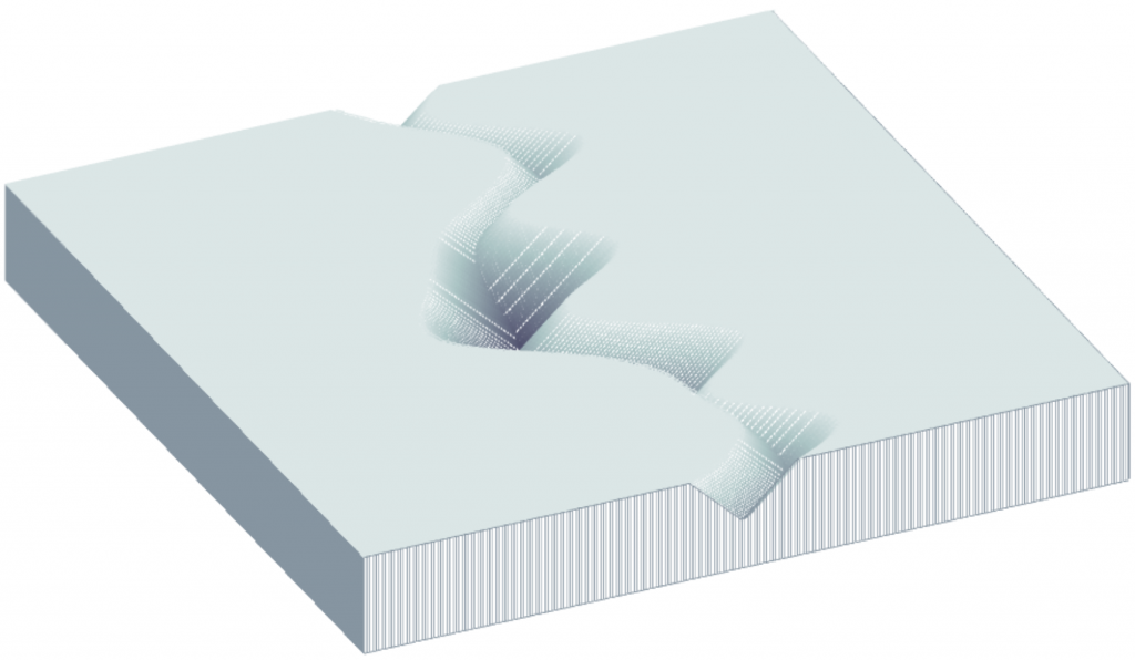
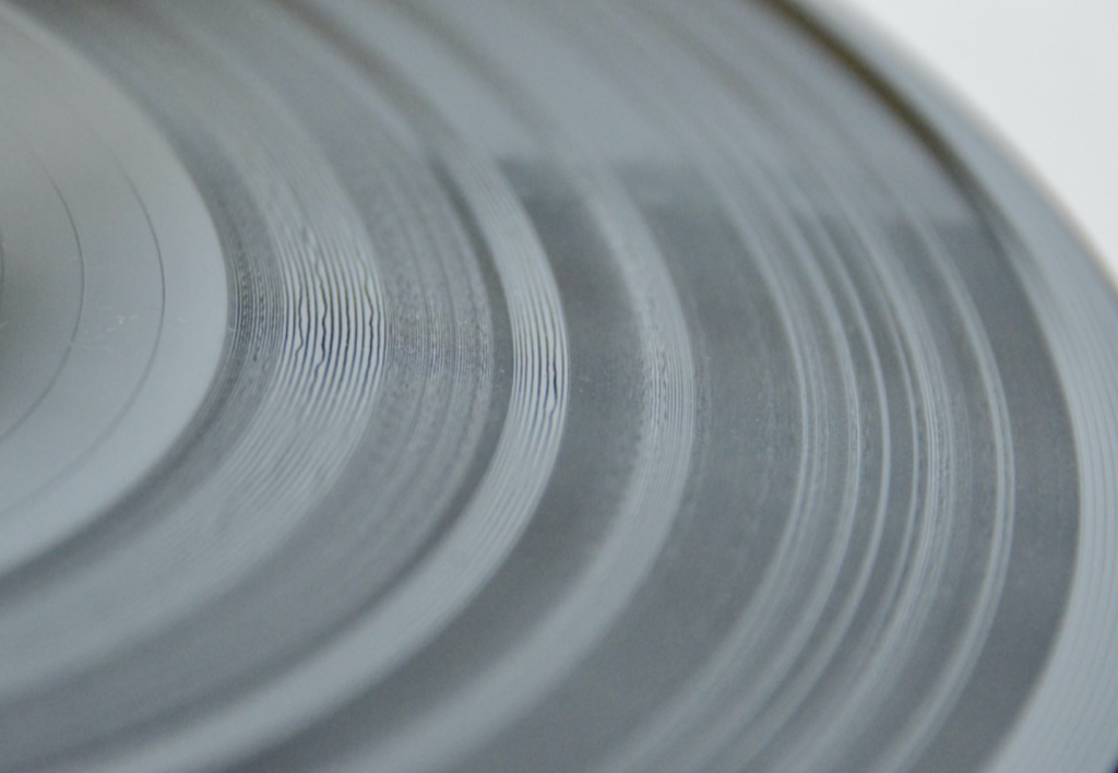
Of course, the higher the modulation velocity of the stylus, the higher the output of the turntable. However, this would also mean that the groove on the vinyl disc would require more space, since it is being modulated more. This means that there is a relationship between the total playing time of a vinyl disc and the modulation velocity. In order to have 20 minutes of music on a 12” LP spinning at 33 1/3 RPM, then it the standard method was to cut 225 “lines per inch” or “LPI” (about 89 lines per centimetre) on the disc. If a mastering engineer wishes to have a signal with a higher output, then the price is a lower playing time (because the grooves much be spaced further apart to accommodate the higher modulation velocity) however, in well-mastered recordings, this spacing is varied according to the dynamic range of the audio signal. In fact, in some classical recordings, it is easy to see the louder passages in the music because the grooves are intentionally spaced further apart, as is illustrated in Figure 3.

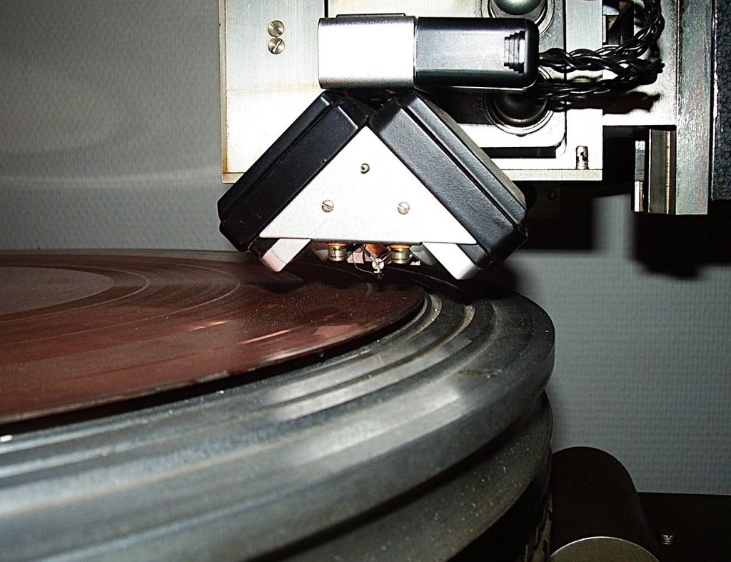
A large part of the performance of a turntable is dependent on the physical contact between the surface of the vinyl and the tip of the stylus. In general terms, as we’re already seen, there is a groove with two walls that vary in height, almost independently and the tip of the stylus traces that movement accordingly. However, it is necessary to get down to the microscopic level to consider this behaviour in more detail.

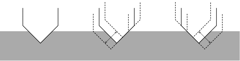
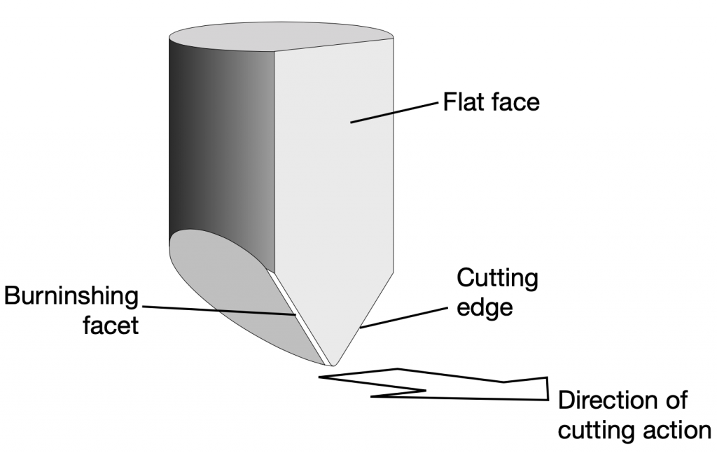
When a record is mastered (meaning, when the master disc is created on a lathe) the groove is cut by a heated stylus that has a specific shape, shown in Figure4. The depth of the groove can range from a minimum of 25 µm to a maximum of 127µm, which, in turn varies the width of the groove.(3)

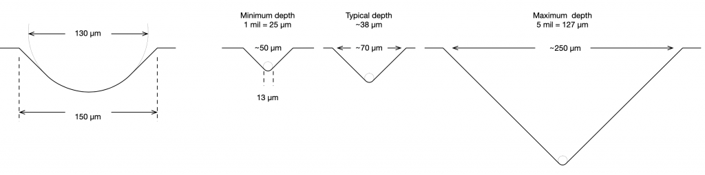
The result is a groove with a varying width and depth that are dependent on the decisions made by the mastering engineer, and a modulation displacement (the left/right size of the “wiggle”) that is dependent on the level of the audio signal that is being reproduced.

In a perfect situation, the stylus that is used to play that signal back on a turntable would have exactly the same shape as the cutting stylus, since this would mean that the groove is traced in exactly the same way that it was cut. This, however, is not practical for a number of reasons. As a result, there are a number of options when choosing the shape of the playback stylus.

Footnotes

1. The assumption here is that the distortion produces harmonics of the signal, which is a simplified view of the truth, but an effect that is easy to measure.
2. (35.4*2) / sqrt(2) because the two channels are modulated at an angle of 45 degrees to the surface of the disc.
3. See “The High-fidelity Phonograph Transducer” B.B. Bauer, JAES 1977 Vol 25, Number 10/11, Oct/Nov 1977

On to Part 4

Back to Part 1: History

The physics

Amplitude vs. Velocity

At the end of Part 1, I mentioned that there is an interaction between magnetic fields, movement, and electrical current. This is at the heart of almost every modern turntable. As the stylus or “needle” (1) is pulled through the grove in the vinyl surface, it moves from side-to-side at a varying speed called the modulation velocity or just the velocity. An example of this wavy groove can be seen in the photo below. Inside the housing of most cartridges are small magnets and coils of wire, either of which is being moved by the stylus as it vibrates. That movement generates an electrical current that is analogous to the shape of the groove: the higher the velocity of the stylus, the higher the electrical signal from the cartridge.

However, this introduces a problem because if the amplitude remains the same at all frequencies the modulation velocity of the stylus decreases with frequency; in other words, the lower the note, the lower the output level, and therefore the less bass. This is illustrated in the graph in Figure 2 below in which three sine waves are shown with different frequencies. The blue line shows the lowest frequency and the orange line is the highest. Notice that all three have the same amplitude (the same maximum “height”). However, if you look at the slopes of the three curves when they pass Time = 0 ms, you’ll see that the higher the frequency, the higher the slope of the line, and therefore the higher the velocity of the stylus.

In order to achieve a naturally flat frequency response from the cartridge, where all frequencies have the same electrical output level, it is necessary to ensure that they have the same modulation velocity, as shown in Figure 3 below. In that plot, it can be seen that the slopes of the three waves are the same at Time = 0 ms. However, it is also evident that, when this is true, they have very different amplitudes: in fact, the amplitude would have to double for every halving of frequency (a drop of 1 octave). This is not feasible, since it would mean that the stylus would have to move left and right by (relatively) huge distances in order to deliver the desired output. For example, if the stylus were moving sideways by $\pm$ 0.1 mm at 1,000 Hz to deliver a signal, then it would have to move $\pm$ 1 mm at 100 Hz, and $\pm$ 10 mm at 10 Hz to deliver the same output level. This is not possible (or at least it’s very impractical).

The solution for this limitation was to use low-frequency audio compensation filters, both at the recording and the playback stages. When a recording is mastered to be cut on a disc, the low frequency level is decreased; the lower the frequency, the lower the level. This results in a signal recorded on disc with a constant amplitude for signals below approximately 1 kHz.

Of course, if this signal were played back directly, there would be an increasing loss of level at lower and lower frequencies. So, to counteract this, a filter is applied to the output signal of the turntable that boosts the low frequencies signals to their original levels.

Surface noise

A second problem that exists with vinyl records is that of dust and dirt. If you look again at the photo in the first Figure at the top of this posting, you can see white specks lodged in the groove. These look very small to us, however, to the stylus, they are very large bumps that cause the tip to move abruptly, and therefore quickly. Since the output signal is still proportional to the modulation velocity, then this makes the resulting cracks and pops quite loud in relation to the audio signal.

In order to overcome this problem, a second filter is used, this time for higher frequencies. Upon playback, the level of the treble is reduced; the higher the frequency the lower the output. This reduces the problem of noise caused by surface dirt on the disc, however it would also reduce the high frequency content of the audio signal itself. This is counteracted by increasing the level of the high-frequency portion of the audio signal when it is mastered for the disc.

This general idea of lowering the level of low-frequencies and/or boosting highs when recording and doing the opposite upon playback is a very old idea in the audio industry and has been used on many formats ranging from film “talkies” to early compact discs. Unfortunately, however, different recording companies and studios used different filters on phonographs for many years. (2) Finally, in the mid-1950s, the Recording Industry Association of America (the RIAA) suggested a standard filter description with the intention that it would be used world-wide for all PVC “vinyl” records.

The two figures below show the responses of the RIAA filters used in both the mastering and the playback of long playing vinyl records. Although there are other standards with slightly different responses, the RIAA filter is by far the most commonly-used.

It may be of interest to note that typical descriptions of the RIAA equalisation filter define the transition points as time constants instead of frequencies. So, instead of 50 Hz, 500 Hz, and 2122 Hz (as shown in the response plots), the points are listed as 3180 µs (microseconds), 318 µs, and 75 µs instead. If you wish to convert a time constant (Tc) to the equivalent frequency (F), you can use the equation below.

F = 1 / (2 π Tc)

Mono to Stereo

In Edison’s first cylinder recordings, the needle vibrated up and down instead of left and right to record the audio signal. This meant that the groove cut into the surface of the tin foil was varying in depth, and therefore in width, as shown in the figure below.

There are some disadvantages to this system, such as the risk of the needle slipping out of the groove when it is too shallow, or suffering from excessive wear if the groove is too deep. In addition, any vertical variation in the recording surface (such as a cylinder that is not quite round, or mechanical vibrations in the player caused by footsteps in the room) becomes translated into unwanted noises upon playback. (3)

Berliner’s Gramophone used a different system, where the needle vibrated sideways instead. This lateral cut system produced a groove on the disc with a constant depth, thus avoiding some of the problems incurred by the vertical cut recording system.

However, both of these systems were only capable of recording a single channel of audio information. In order to capture 2-channel stereo audio (invented by Alan Blumlein in 1931) the system had to be adapted somehow. The initial challenge was to find a way of making a disc player that could reproduce two channels of stereo audio, while still maintaining compatibility with lateral-cut discs.

The solution was to rotate the modulation direction by 45 degrees, so the two walls of the groove are used to record the two separate audio channels. This means that the stylus moves in two (theoretically independent) axes as shown in the figure below. When the same signal is applied to both channels (better known as a “dual-mono” or “in-phase” signal), then the stylus moves upwards for the left while moving downwards for the right channel (or down-left & up-right), for example. This means that signals that are identical in both channels move the stylus laterally, exactly as in earlier monophonic discs. (For a more correct explanation of this movement, see this webpage)

As a result, if you look at the groove in a modern two-channel stereo LP, it appears first glance that it simply wiggles left-to-right. However, if you inspect the same groove with extreme magnification, you can see that the modulations in the two sidewalls of the groove are slightly different, since the audio signals on the left and right channels are not identical.

Footnotes

1. Some authors reserve the term “stylus” for the device that is used to cut the groove during mastering, and the term “needle” for the device used to play a phonographic record. However, I’ll use the two terms interchangeably in this series.
2. See the Manual of Analogue Sound Restoration Techniques (2008), by Peter Copeland
3. Some 78 RPM discs use a vertical cutting system as well, including those made by Edison Disc Records and Pathé.

On to Part 3