Let’s go back to something I said in the last post:
Mistake #1
I just jumped to at least three conclusions (probably more) that are going to haunt me.
The first was that my “digital audio system” was something like the following:
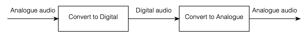
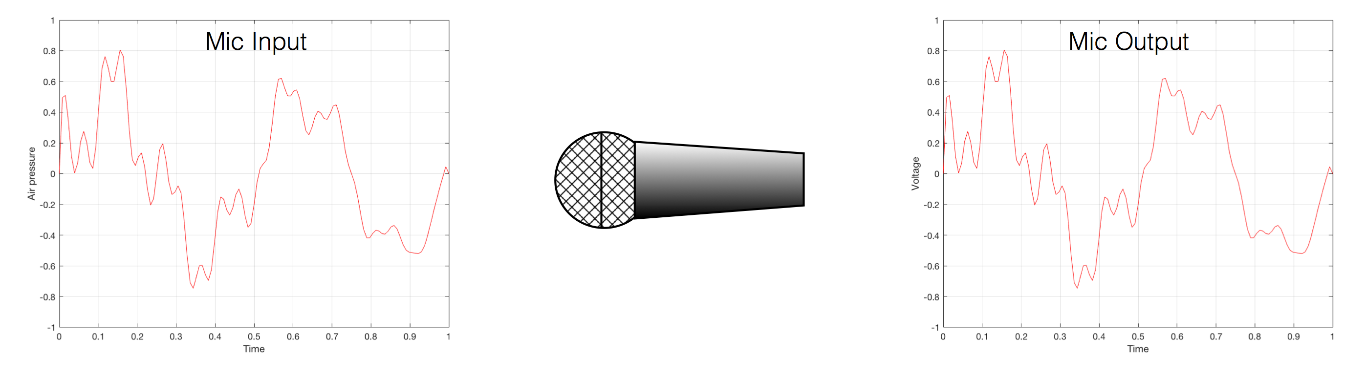
As you can see there, I took an analogue audio signal, converted it to digital, and then converted it back to analogue. Maybe I transmitted it or stored it in the part that says “digital audio”.
However, the important, and very probably incorrect assumption here is that I did nothing to the signal. No volume control, no bass and treble adjustments… nothing.
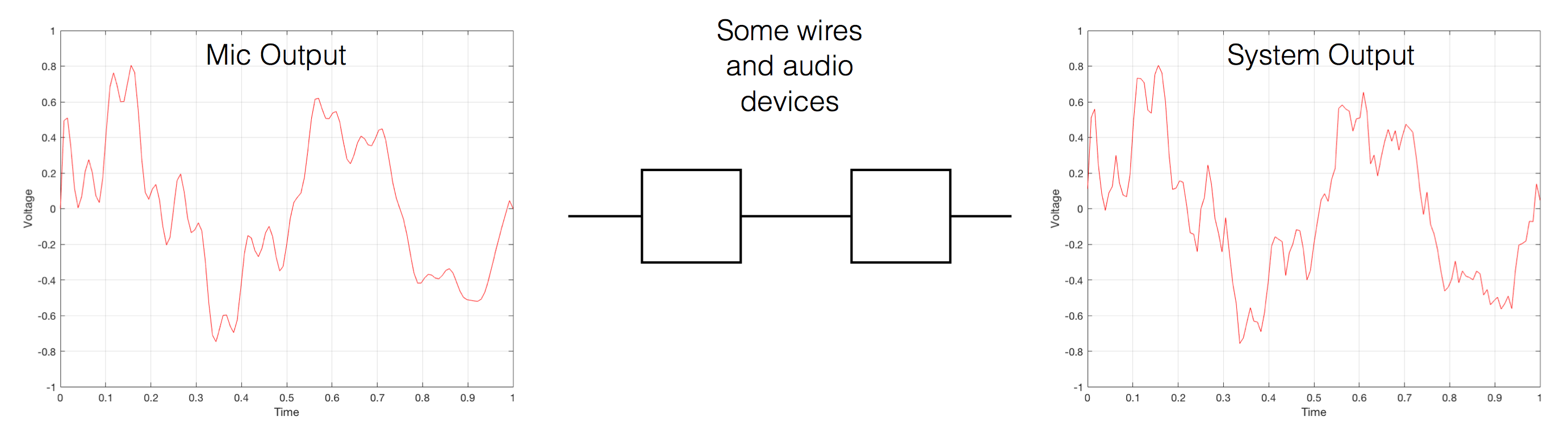
If you consider that signal flow from the position of an end-consumer playing a digital recording, this was pretty easy to accomplish in the “old days” when we were all playing CDs. That’s because (in a theoretical, oversimplified world…)
- the output of the mixing/mastering console was analogue
- that analogue signal was converted to digital in the mastering studio
- the resulting bits were put on a disc
- you put that disc in your player which contained a DAC that converted the signal directly to analogue
- you then sent the signal to your “processing” (a.k.a. “volume control”, and maybe some bass and treble adjustment.).
So, that flowchart in Figure 1 was quite often true in 1985.
These days, things are probably VERY different… These days, the signal path probably looks something more like this (note that I’ve highlighted “alterations” or changes in the bits in the audio signal in red):
- The signal was converted from analogue to digital in the studio
(yes, I know… studios often work with digital mixers these days, but at least some of the signals within the mix were analogue to start – unless you are listening to music made exclusively with digital synthesizers) - The resulting bits were saved on a file
- Depending on the record label, the audio signal was modified to include a “watermark” that can identify it later – in court, when you’ve been accused of theft.
- The file was transferred to a storage device (let’s say “hard drive”) in a large server farm renting out space to your streaming service
- The streaming service encodes the file
- If the streaming service does not offer an lossless option, then the file is converted to a lossy format like MP3, Ogg Vorbis, AAC, or something else.
- If the streaming service offers a lossless option, then the file is compressed using a format like FLAC or ALAC (This is not an alteration, since, with a lossless compression system, you don’t lose anything)
- You download the file to your computer
(it might look like an audio player – but that means it’s just a computer that you can’t use to check your social media profile) - You press play, and the signal is decoded (either from the lossy CODEC or the compression format) back to LPCM. (Still not an alteration. If it’s a lossy CODEC, then the alteration has already happened.)
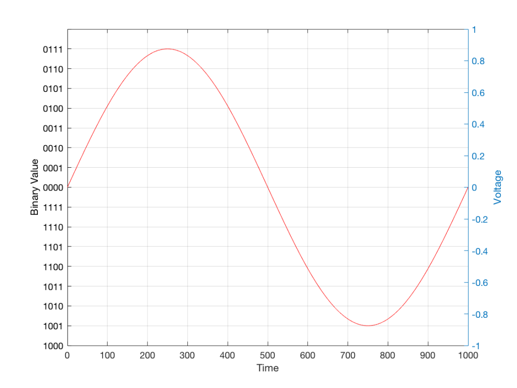
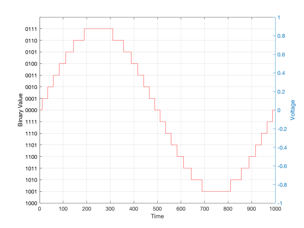
- That LPCM signal might be sample-rate converted
- The streaming service’s player might do some processing like dynamic range compression or gain changes if you’ve asked it to make all the songs have the same level.
- All of the user-controlled “processing” like volume controls, bass, and treble, are done to the digital signal.
- The signal is sent to the loudspeaker or headphones
- If you’re sending the signal wirelessly to a loudspeaker or headphones, then the signal is probably re-encoded as a lossy CODEC like AAC, aptX, or SBC.
(Yes, there are exceptions with wireless loudspeakers, but they are exceptions.)
- If you’re sending the signal as a digital signal over a wire (like S/PDIF or USB), the you get a bit-for-bit copy at the input of the loudspeaker or headphones.
- If you’re sending the signal wirelessly to a loudspeaker or headphones, then the signal is probably re-encoded as a lossy CODEC like AAC, aptX, or SBC.
- The loudspeakers or headphones might sample-rate convert the signal
- The sound is (finally) converted to analogue – either one stream per channel (e.g. “left”) or one stream per loudspeaker driver (e.g. “tweeter”) depending on the product.
So, as you can see in that rather long and complicated list (it looks complicated, but I’ve actually simplified it a little, believe it or not), there’s not much relation to the system you had in 1985.
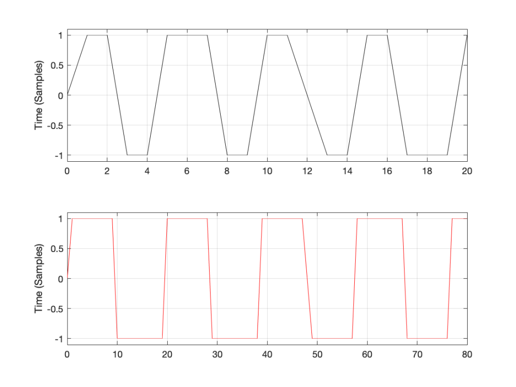
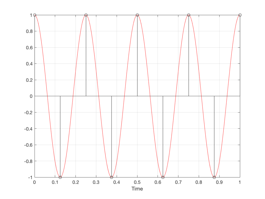
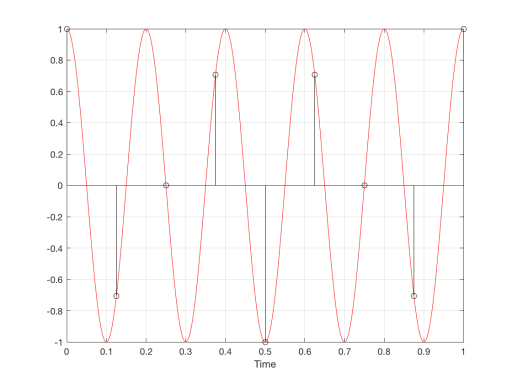
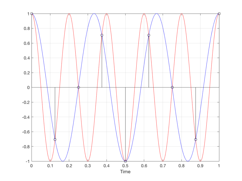
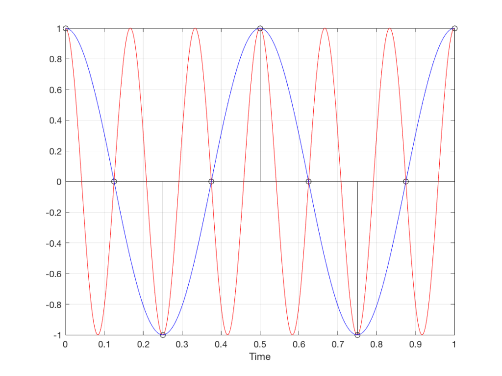
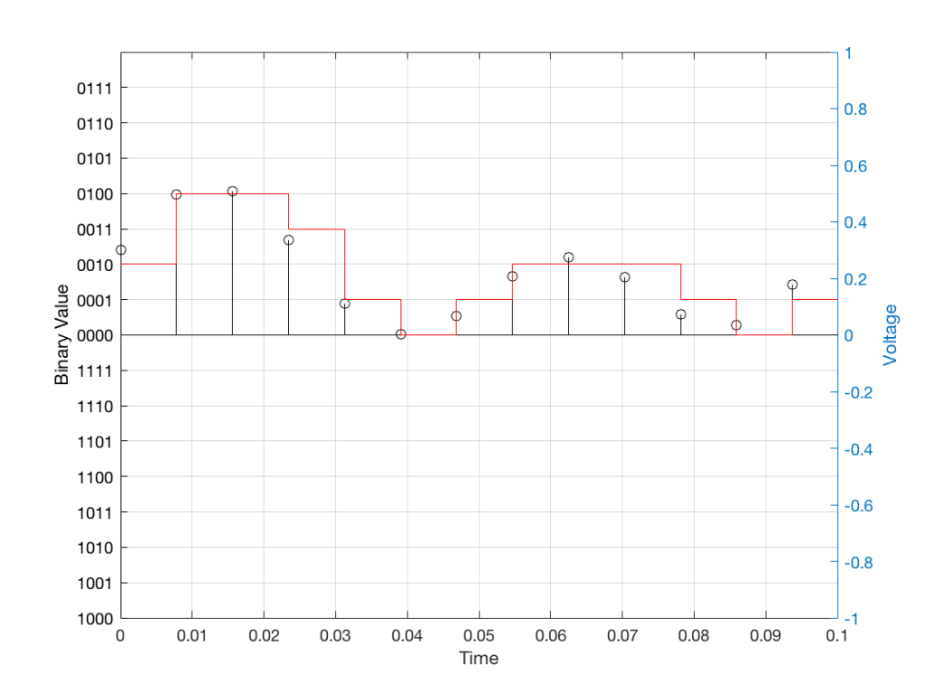
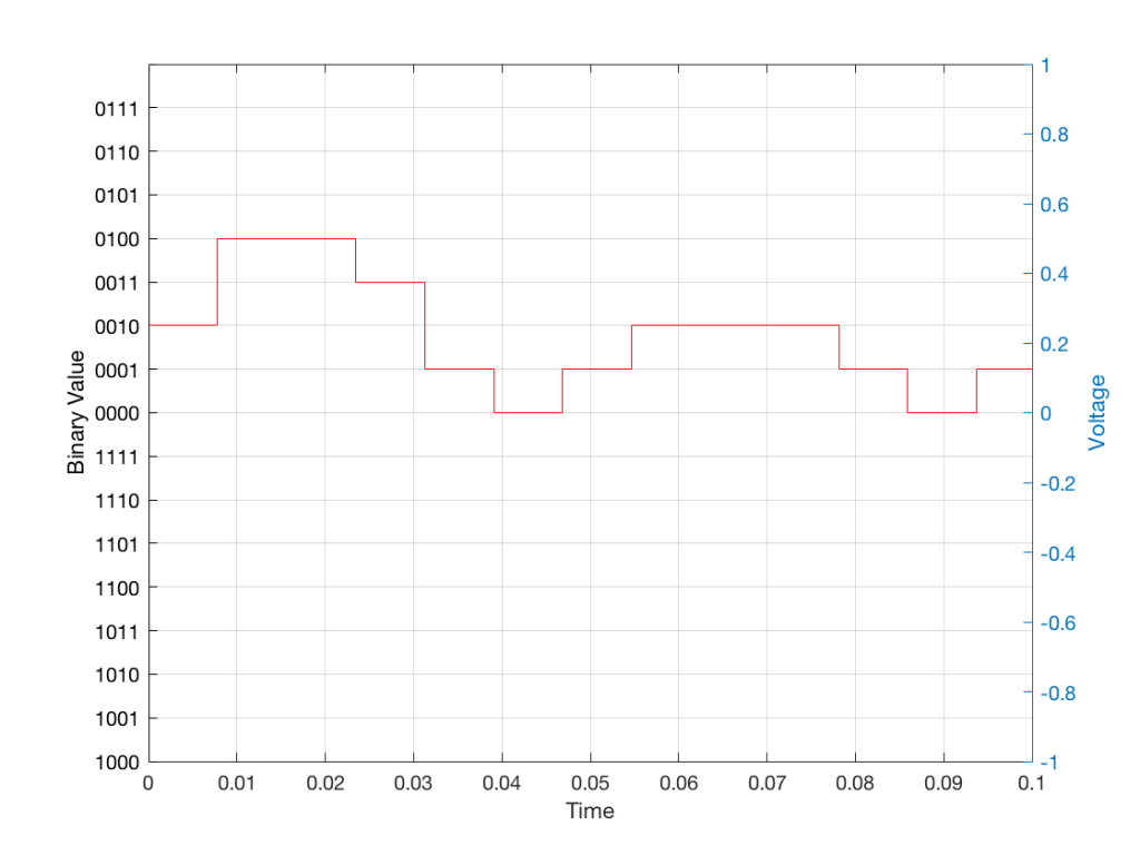
Let’s take just one of those blocks and see what happens if things go horribly wrong. I’ll take the “volume control” block and add some distortion to see the result with two LPCM systems that have two different sampling rates, one running at 48 kHz and the other at 194 kHz – four times the rate. Both systems are running at 24 bits, with TPDF dither (I won’t explain what that means here). I’ll start by making a 10 kHz tone, and sending it through the system without any intentional distortion. If we look at those two signals in the time domain, they’ll look like this:
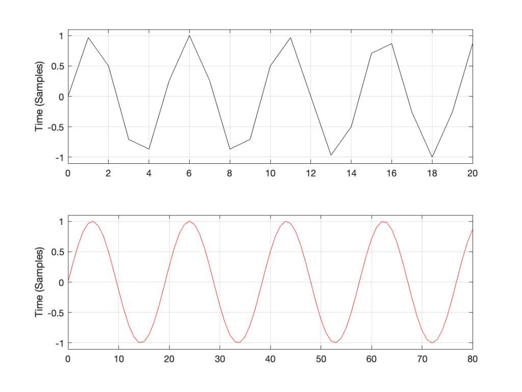
The sine tone in the 48 kHz system may look less like a sine tone than the one in the 192 kHz system, however, in this case, appearances are deceiving. The reconstruction filter in the DAC will filter out all the high frequencies that are necessary to reproduce those corners that you see here, so the resulting output will be a sine wave. Trust me.
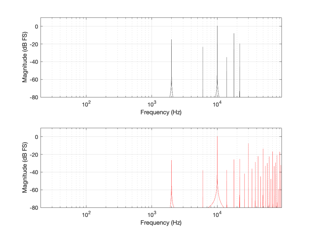
If we look at the magnitude responses of these two signals, they look like Figure 2, below.
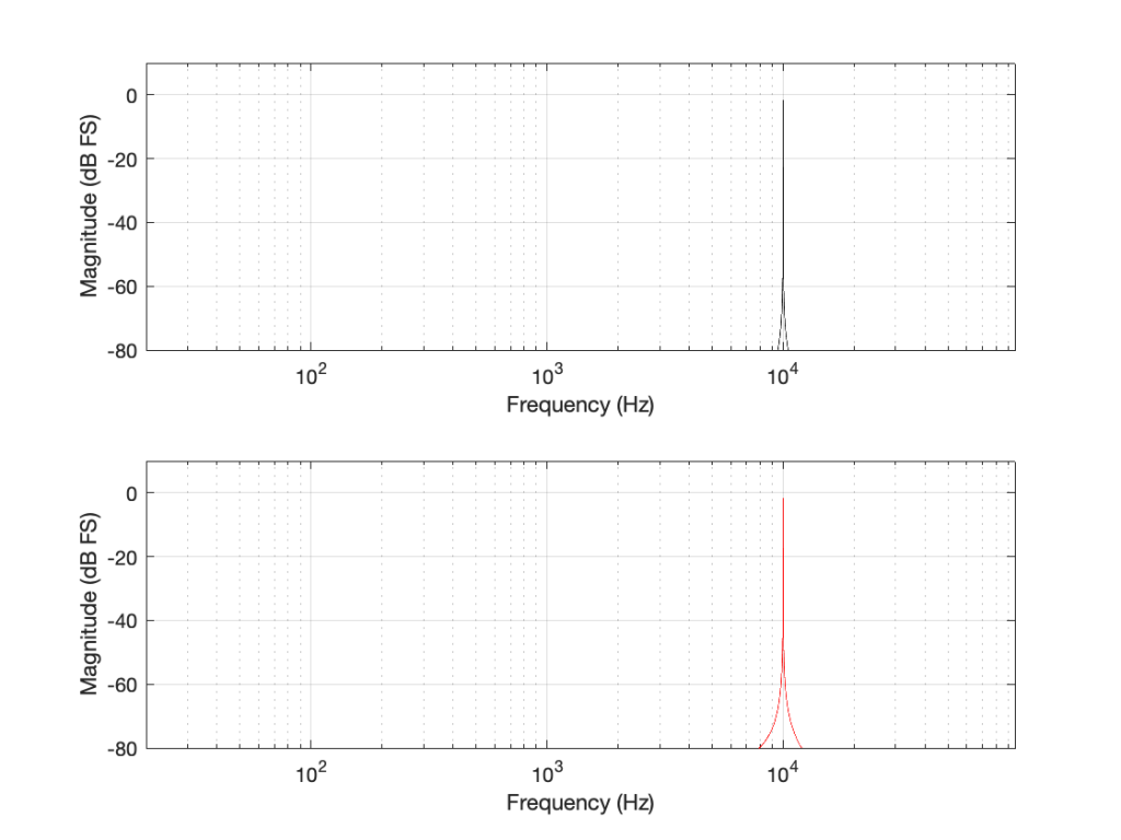
You may be wondering about the “skirts” on either side of the 10 kHz spikes. These are not really in the signal, they’re a side-effect (ha ha) of the windowing process used in the DFT (aka FFT). I will not explain this here – but I did a long series of articles on windowing effects with DFTs, so you can search for it if you’re interested in learning more about this.
If you’re attentive, you’ll notice that both plots extend up to 96 kHz. That’s because the 192 kHz system on the bottom has a Nyquist frequency of 96 kHz, and I want both plots to be on the same scale for reasons that will be obvious soon.
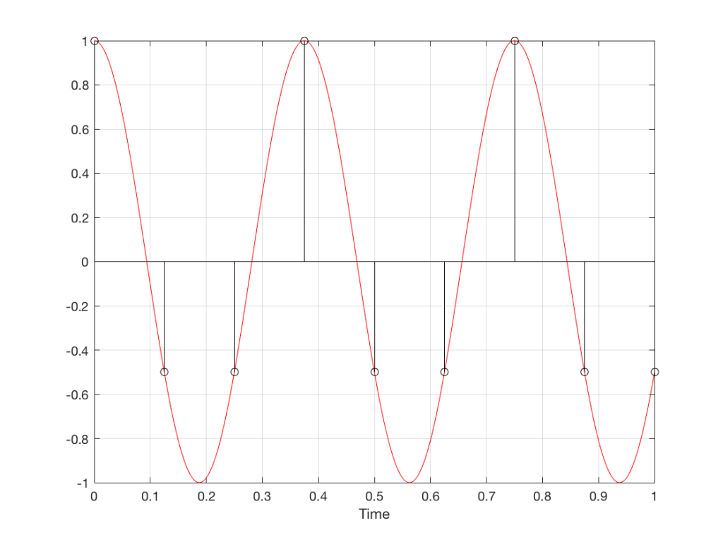
Now I want to make some distortion. In order to make things obvious, I’m going to make a LOT of distortion. I’ve made the sine wave try to have an amplitude that is 10 times higher than my two systems will allow. In other words, my amplitude should be +/- 10, but the signal clips at +/- 1, resulting in something looking very much like a square wave, as shown in Figure 3.
You may already know that if you want to make a square wave by building it up using its constituent harmonics, you need to have the fundamental (which we’ll call Fc. In our case, Fc = 10 kHz) with an amplitude that we’ll say is “A”, you then add the
- 3rd harmonic (3 times Fc, so 30 kHz in our case) with an amplitude of A/3.
- 5th harmonic (5 Fc = 50 kHz) with an amplitude of A/5
- 7 Fc at A/7
- and so on up to infinity
Let’s look at the magnitude responses of the two signals above to see if that’s true.
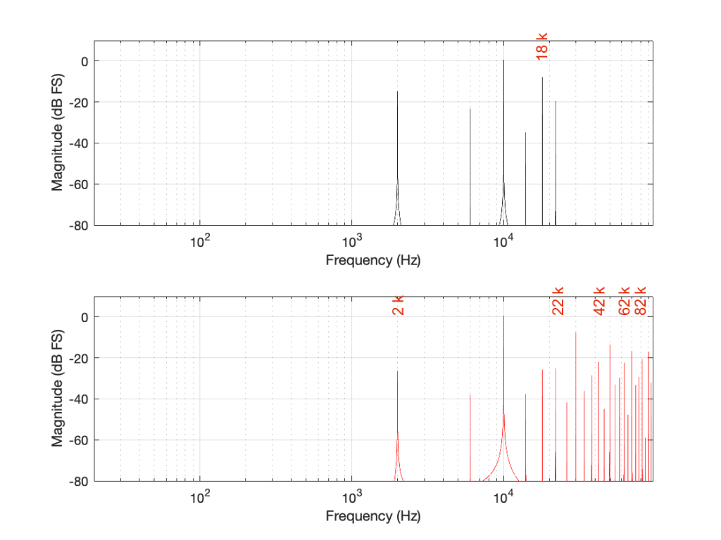
If we look at the bottom plot first (running at 192 kHz and with a Nyquist limit of 96 kHz) the 10 kHz tone is still there. We can also see the harmonics at 30 kHz, 50 kHz, 70 kHz, and 90 kHz in amongst the mess of other spikes we’ll get to those soon…)
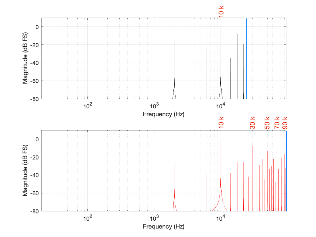
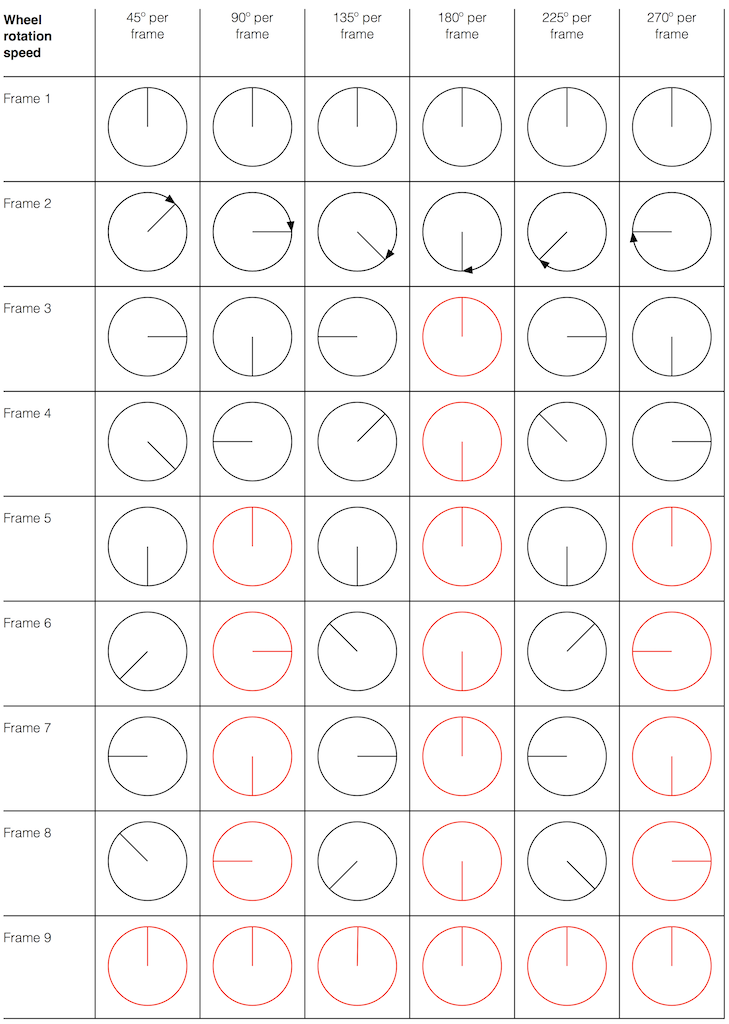
Looking at the top plot (running at 48 kHz and with a Nyquist limit of 24 kHz), we see the 10 kHz tone, but the 30 kHz harmonic is not there – because it can’t be. Signals can’t exist in our system above the Nyquist limit. So, what happens? Think back to the images of the rotating wheel in Part 3. When the wheel was turning more than 1/2 a turn per frame of the movie, it appears to be going backwards at a different speed that can be calculated by subtracting the actual rotation from 180º (half-a-turn).
The same is true when, inside a digital audio signal flow, we try to make a signal that’s higher than Nyquist. The energy exists in there – it just “folds” to another frequency – its “alias”.
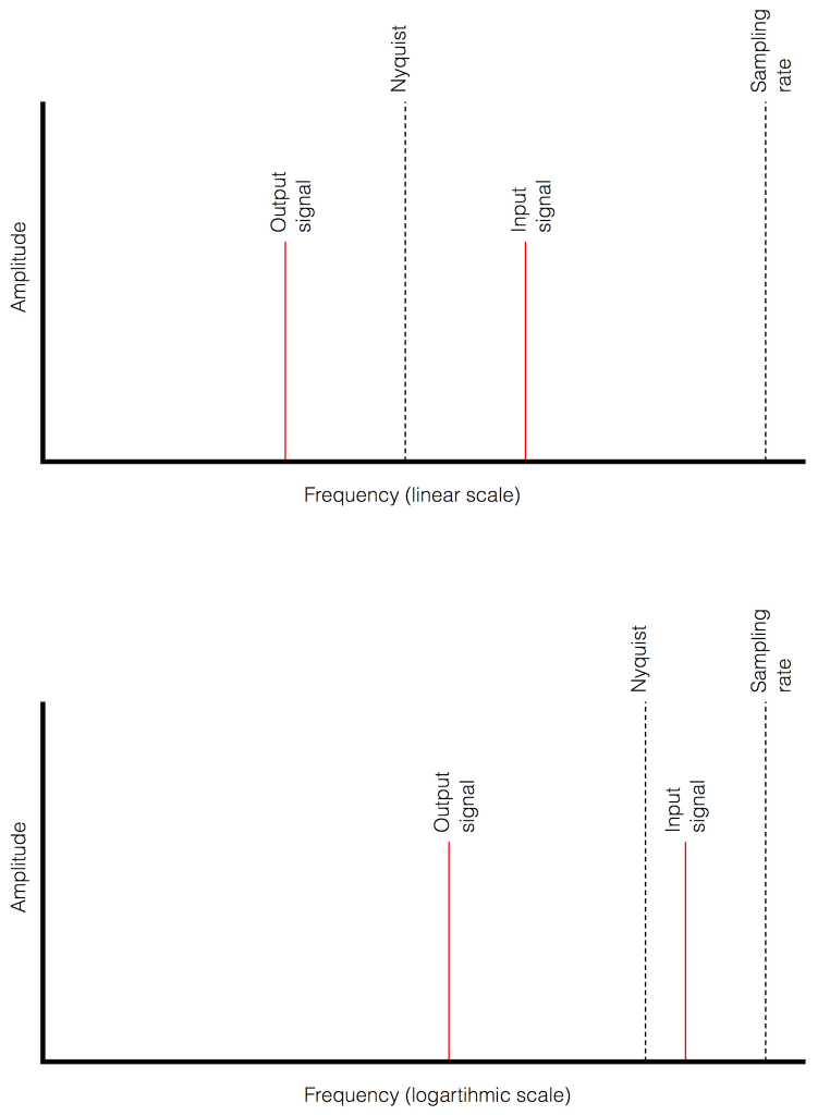
We can look at this generally using Figure 6.
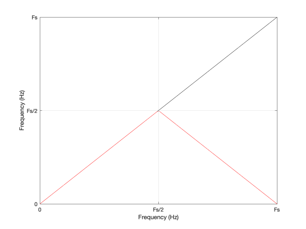
Looking at Figure 6: If we make a sine tone that sweeps upward from 0 Hz to the Nyquist frequency at Fs/2 (half the sampling rate or sampling frequency) then the output is the same as the input. However, when the intended frequency goes above Fs/2, the actual frequency that comes out is Fs/2 minus the intended frequency. This creates a “mirror” effect.
If the intended frequency keeps going up above Fs, then the mirroring happens again, and again, and again… This is illustrated in Figure 7.
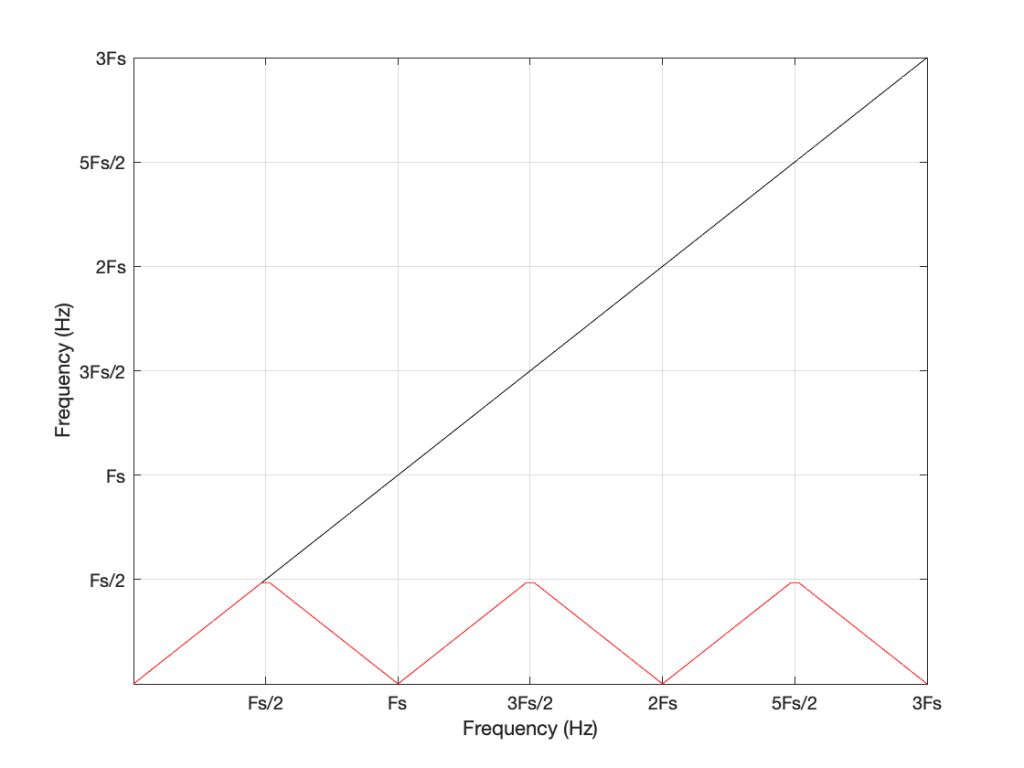
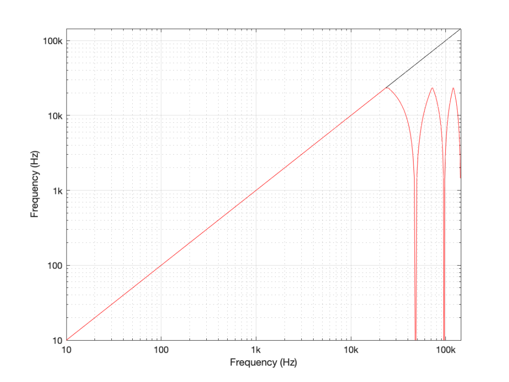
This plot is shown with linear scales for both the X- and Y-axes to make it easy to understand. If the axes in Figure 7 were scaled to a logarithmic scaling instead (which is how “Frequency Response” are normally shown, since this corresponds to how we hear frequency differences), then it would look like Figure 8.
Coming back to our missing 30 kHz harmonic in the 48 kHz LPCM system: Since 30 kHz is above the Nyquist limit of 24 kHz in that system, it mirrors down to 24 kHz – (30 kHz – 24 kHz) = 18 kHz. The 50 kHz harmonic shows up as an alias at 2 kHz. (follow the red line in Figure 7: A harmonic on the black line at 48 kHz would actually be at 0 Hz on the red line. Then, going 2000 Hz up to 50 kHz would bring the red line up to 2 kHz.)
Similarly, the 110 kHz harmonic in the 192 kHz system will produce an alias at 96 kHz – (110 kHz – 96 kHz) = 82 kHz.
If I then label the first set of aliases in the two systems, we get Figure 9.
Now we have to stop for a while and think about what’s happened.
We had a digital signal that was originally “valid” – meaning that it did not contain any information above the Nyquist frequency, so nothing was aliasing. We then did something to the signal that distorted it inside the digital audio path. This produced harmonics in both cases, however, some of the harmonics that were produced are harmonically related to the original signal (just as they ought to be) and others are not (because they’re aliases of frequency content that cannot be reproduced by the system.
What we have to remember is that, once this happens, that frequency content is all there, in the signal, below the Nyquist frequency. This means that, when we finally send the signal out of the DAC, the low-pass filtering performed by the reconstruction filter will not take care of this. It’s all part of the signal.
So, the question is: which of these two systems will “sound better” (whatever that means)? (I know, I know, I’m asking “which of these two distortions would you prefer?” which is a bit of a weird question…)
This can be answered in two ways that are inter-related.
The first is to ask “how much of the artefact that we’ve generated is harmonically related to the signal (the original sine tone)?” As we can see in Figure 5, the higher the sampling rate, the more artefacts (harmonics) will be preserved at their original intended frequencies. There’s no question that harmonics that are harmonically related to the fundamental will sound “better” than tones that appear to have no frequency relationship to the fundamental. (If I were using a siren instead of a constant sine tone, then aliased harmonics are equally likely to be going down or up when the fundamental frequency goes up… This sounds weird.)
The second is to look at the levels of the enharmonic artefacts (the ones that are not harmonically related to the fundamental). For example, both the 48 kHz and the 192 kHz system have an aliased artefact at 2 kHz, however, its level in the 48 kHz system is 15 dB below the fundamental whereas, in the 192 kHz system, it’s more than 26 dB below. This is because the 6 kHz artefact in the 48 kHz system is an alias of the 30 kHz harmonic, whereas, in the 192 kHz system, it’s an alias of the 190 kHz harmonic, which is much lower in level.
As I said, these two points are inter-related (you might even consider them to be the same point) however, they can be generalised as follows:
The higher the sampling rate, the more the artefacts caused by distortion generated within the system are harmonically related to the signal.
In other words, it gives a manufacturer more “space” to screw things up before they sound bad. The title of this posting is “Mirrors are bad” but maybe it should be “Mirrors are better when they’re further away” instead.
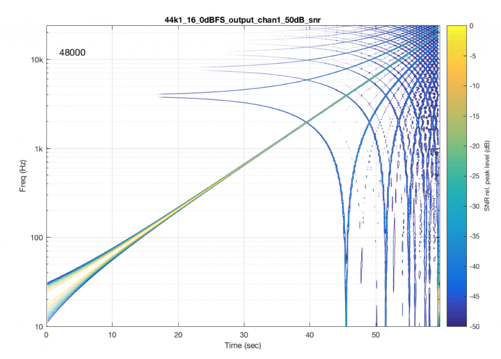
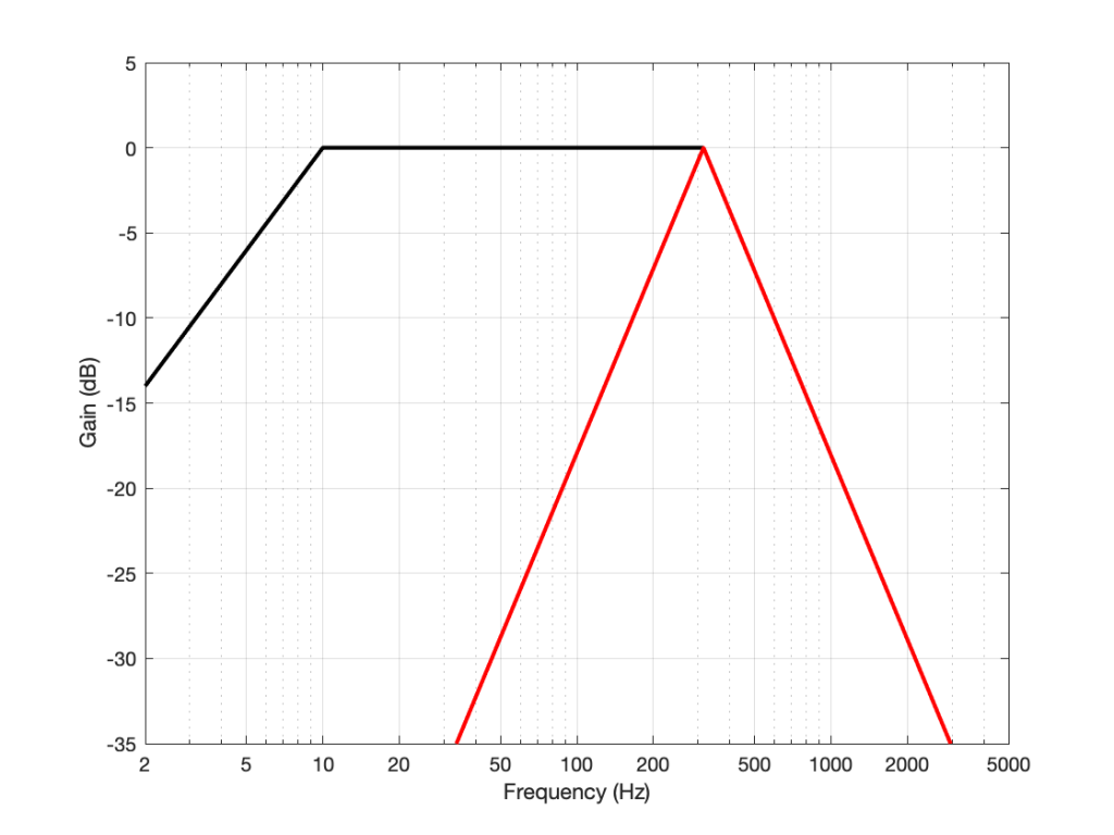
Of course, the distortion that’s actually generated by processing inside a digital audio system (hopefully) won’t be anything like the clipping that I did to the signal. On the other hand, I’ve measured some systems that exhibit exactly this kind of behaviour. I talked about this in another series about Typical Problems in Digital Audio: Aliasing where I showed this measurement of a real device:
However, I’m not here to talk about what you can or can’t hear – that is dependent on too many variables to make it worth even starting to talk about. The point of this series is not to prove that something is better or worse than something else. It’s only to show the advantages and disadvantages of the options so that you can make an informed choice that best suits your requirements.


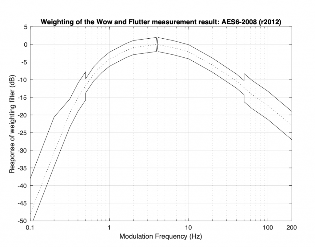

 is the harmonic distortion in percent,
  is the angular frequency of the modulation caused by the audio signal (calculated using
  ),
),  is the peak amplitude in mm,
  is the tracking error in degrees,
  is the angular frequency of rotation (the speed of the record in radians per second. For example, at 33 1/3 RPM,
  ) and
) and  is the radius (the distance of the groove from the centre of the disk). (see “Tracking Angle in Phonograph Pickups” by B.B. Bauer, Electronics (March 1945))