The original Loudness War

The June, 1968 issue of Wireless World magazine includes an article by R.T. Lovelock called “Loudness Control for a Stereo System”. This article partly addresses the issue of resistance behaviour one or more channels of a variable resistor. However, it also includes the following statement:

It is well known that the sensitivity of the ear does not vary in a linear manner over the whole of the frequency range. The difference in levels between the threshold of audibility and that of pain is much less at very low and very high frequencies than it is in the middle of the audio spectrum. If the frequency response is adjusted to sound correct when the reproduction level is high, it will sound thin and attenuated when the level is turned down to a soft effect. Since some people desire a high level, while others cannot endure it, if the response is maintained constant while the level is altered, the reproduction will be correct at only one of the many preferred levels. If quality is to be maintained at all levels it will be necessary to readjust the tone controls for each setting of the gain control

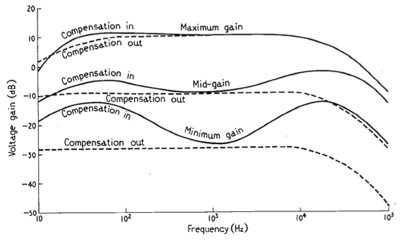
The article includes a circuit diagram that can be used to introduce a low- and high-frequency boost at lower settings of the volume control, with the following example responses:

These days, almost all audio devices include some version of this kind of variable magnitude response, dependent on volume. However, in 1968, this was a rather new idea that generated some debate.

In the following month’s issue The Letters to the Editor include a rather angry letter from John Crabbe (Editor of Hi-Fi News) where he says

Mr. Lovelock’s article in your June issue raises an old bogey which I naively thought had been buried by most British engineers many years ago. I refer, not to the author’s excellent and useful thesis on achieving an accurate gain control law, but to the notion that our hearing system’s non-linear loudness / frequency behaviour justifies an interference with response when reproducing music at various levels.

Of course, we all know about Fletcher-Munson and Robinson-Dadson, etc, and it is true that l.f. acuity declines with falling sound pressure level; though the h.f. end is different, and latest research does not support a general rise in output of the sort given by Mr. Lovelock’s circuit. However, the point is that applying the inverse of these curves to sound reproduction is completely fallacious, because the hearing mechanism works the way it does in real life, with music loud or quiet, and no one objects. If `live’ music is heard quietly from a distant seat in the concert hall the bass is subjectively less full than if heard loudly from the front row of the stalls. All a `loudness control’ does is to offer the possibility of a distant loudness coupled with a close tonal balance; no doubt an interesting experiment in psycho-acoustics, but nothing to do with realistic reproduction.

In my experience the reaction of most serious music listeners to the unnaturally thick-textured sound (for its loudness) offered at low levels by an amplifier fitted with one of these abominations is to switch it out of circuit. No doubt we must manufacture things to cater for the American market, but for goodness sake don’t let readers of Wireless World think that the Editor endorses the total fallacy on which they are based.

with Lovelock replying:

Mr. Crabbe raises a point of perennial controversy in the matter of variation of amplifier response with volume. It was because I was aware of the difference in opinion on this matter that a switch was fitted which allowed a variation of volume without adjustment of frequency characteristic. By a touch of his finger the user may select that condition which he finds most pleasing, and I still think that the question should be settled by subjective pleasure rather than by pure theory.

and

Mr. Crabbe himself admits that when no compensation is coupled to the control, it is in effect a ‘distance’ control. If the listener wishes to transpose himself from the expensive orchestra stalls to the much cheaper gallery, he is, of course, at liberty to do so. The difference in price should indicate which is the preferred choice however.

In the August edition, Crabbe replies, and an R.E. Pickvance joins the debate with a wise observation:

In his article on loudness controls in your June issue Mr. Lovelock mentions the problem of matching the loudness compensation to the actual sound levels generated. Unfortunately the situation is more complex than he suggests. Take, for example, a sound reproduction system with a record player as the signal source: if the compensation is correct for one record, another record with a different value of modulation for the same sound level in the studio will require a different setting of the loudness control in order to recreate that sound level in the listening room. For this reason the tonal balance will vary from one disc to another. Changing the loudspeakers in the system for others with different efficiencies will have the same effect.

In addition, B.S. Methven also joins in to debate the circuit design.

The debate finally peters out in the September issue.

Apart from the fun that I have reading this debate, there are two things that stick out for me that are worth highlighting:

  • Notice that there is a general agreement that a volume control is, in essence, a distance simulator. This is an old, and very common “philosophy” that we forget these days.
  • Pickvance’s point is possibly more relevant today than ever. Despite the amount of data that we have with respect to equal loudness contours (aka “Fletcher and Munson curves”) there is still no universal standard in the music industry for mastering levels. Now that more and more tracks are being released in a Dolby Atmos-encoded format, there are some rules to follow. However, these are very different from 2-channel materials, which have no rules at all. Consequently, although we know how to compensate for changes in response in our hearing as a function of level, we don’t know what the reference level should be for any given recording.

3-channel vinyl

Another gem of historical information from the Centennial Issue of the JAES in 1977.

This one is from the article titled “The Recording Industry in Japan” by Toshiya Inoue of the Victor Company of Japan. In it, you can find the following:

Notice that this describes a 3-channel system developed by the Victor Company using FM with a carrier frequency of 24 kHz and a modulation of ±4kHz to create a third channel on the vinyl. The resulting signal had a bandwidth of 50 Hz to 5 kHz and a SNR of 47 dB.

Interestingly, this was developed from 1961-1965: starting 9 years before CD-4 quadraphonic was introduced to the market, which used the same basic principle of FM modulation to encode the extra channels.

The Sound of Music

This episode of The Infinite Monkey Cage is worth a listen if you’re interested in the history of recording technologies.

There’s one comment in there by Brian Eno that I COMPLETELY agree with. He mentions that we invented a new word for moving pictures: “movies” to distinguish them from the live equivalent, “plays”. But we never really did this for music… Unless, of course, you distinguish listening to a “concert” from listening to a “recording” – but most of us just say “I’m listening to music”.

100-year old upmixer

I had a little time at work today waiting for some visitors to show up and, as I sometimes do, I pulled an old audio book off the shelf and browsed through it. As usually happens when I do this, something interesting caught my eye.

I was reading the AES publication called “The Phonograph and Sound Recording After One-Hundred Years” which was the centennial issue of the Journal of the AES from October / November 1977.

In that issue of the JAES, there is an article called “Record Changers, Turntables, and Tone Arms – A Brief Technical History” by James H. Kogen of Shure Brothers Incorporated, and in that article he mentions US Patent Number 1,468,455 by William H. Bristol of Waterbury, CT, titled “Multiple Sound-Reproducing Apparatus”.

Before I go any further, let’s put the date of this patent in perspective. In 1923, record players existed, but they were wound by hand and ran on clockwork-driven mechanisms. The steel needle was mechanically connected to a diaphragm at the bottom of a horn. There were no electrical parts, since lots of people still didn’t even have electrical wiring in their homes: radios were battery-powered. Yes, electrically-driven loudspeakers existed, but they weren’t something you’d find just anywhere…

In addition, 3- or 2-channel stereo wasn’t invented yet, Blumlein wouldn’t patent a method for encoding two channels on a record until 1931: 8 years in the future…

But, if we look at Bristol’s patent, we see a couple of astonishing things, in my opinion.

If you look at the top figure, you can see the record, sitting on the gramophone (I will not call it a record player or a turntable…). The needle and diaphragm are connected to the base of the horn (seen on the top right of Figure 3, looking very much like my old Telefunken Lido, shown below.

But, below that, on the bottom of Figure 3 are what looks a modern-ish looking tonearm (item number 18) with a second tonearm connected to it (item number 27). Bristol mentions the pickups on these as “electrical transmitters”: this was “bleeding edge” emerging technology at the time.

So, why two pickups? First a little side-story.

Anyone who works with audio upmixers knows that one of the “tricks” that are used is to derive some signal from the incoming playback, delay it, and then send the result to the rear or “surround” loudspeakers. This is a method that has been around for decades, and is very easy to implement these days, since delaying audio in a digital system is just a matter of putting the signal into a memory and playing it out a little later.

Now look at those two tonearms and their pickups. As the record turns, pickup number 20 in Figure 3 will play the signal first, and then, a little later, the same signal will be played by pickup number 26.

Then if you look at Figure 6, you can see that the first signal gets sent to two loudspeakers on the right of the figure (items number 22) and the second signal gets sent to the “surround” loudspeakers on the left (items number 31).

So, here we have an example of a system that was upmixing a surround playback even before 2-channel stereo was invented.

Mind blown…

NB. If you look at Figure 4, you can see that he thought of making the system compatible with the original needle in the horn. This is more obvious in Figures 1 and 2, shown below.

Acoustic measurements: Part 3

In Part 2, I showed the raw magnitude response results of three pairs of headphones measured on three different systems, each done 5 times. However, when you plot magnitude responses on a scale with 80 dB like I did there, it’s difficult to see what’s going on.

Differences in measurements relative to average

One way to get around this issue is to ignore the raw measurement and look at the differences between them, which is what we’ll do here. This allows us to “zoom in” on the variations in the measurements, at the cost of knowing what the general overall responses are.

Figure 1 in Part 2 showed the 5 x 3 sets of raw magnitude responses of the open headphones. I then take each set of 5 measurements (remember that these 5 measurements were done by removing the headphones and re-setting them each time on the measurement rig) and find their average response. Then I plot the difference between each of the 5 measurements and that average, and this is done for each of the three measurement systems, as shown below in Figure 1.

Figure 1: Open headphones: The difference between each of the 5 measurements done on each system and the mean (average) of those 5 measurements.
Figure 2: Semi-open headphones: The difference between each of the 5 measurements done on each system and the mean (average) of those 5 measurements.
Figure 3: Closed headphones: The difference between each of the 5 measurements done on each system and the mean (average) of those 5 measurements.

Some of the things that were intuitively visible in the plots in Part 2 are now obvious:

  • There is a huge change in the measured magnitude response in the high frequency bands, even when the pair of headphones and the measurement rig are the same. This is the result of small changes in the physical position of the headphones on the rig, as well as changes in the clamping force (modified by moving the headband extension). I intentionally made both of these “errors” to show the problem. Notice that the differences here are greater than ±10 dB, which is a LOT.
  • Overall, the differences between the measurements on the dummy head are bigger and have a lower frequency range than for the other two systems. This is mostly due to two things:
    • because the dummy head has pinnae (ears), very small changes in position result in big changes in response
    • it is easier to have small leaks around the ear cushions on a dummy head than with a flat surrounding of a metal plate or an artificial ear. This is the reason for the low-frequency differences with the closed headphones. Leaks have no effect on open headphone designs, since they are always leaking out through the diaphragm itself.

The differences that you can see here are the reason that, when we’re measuring headphones, we never measure just once. We always do a minimum of 5 measurements and look at the average of the set. This is standard practice, both for headphone developers and experienced reviewers like this one, for example.

In addition to this averaging, it’s also smart to do some kind of smoothing (which I have not done here…) to avoid being distracted by sharp changes in the response. Sharp peaks and dips can be a problem, particularly when you look at the phase response, the group delay, or looking for ringing in the time domain. However, it’s important to remember that the peaks and dips that you see in the measurements above might not actually be there when you put the headphones on your head. For example, if the variations are caused by standing waves inside the headphones due to the fact that the measurement system itself is made of reflective plastic or metal (but remember that you aren’t…) then the measurement is correct, but it doesn’t reflect (ha ha…) reality…

One additional thing to remember with these plots is that something that looks like a peak in the curve MIGHT be a peak, but it might also be a dip in the average curve because we’re only looking at the differences in the responses.

System differences

Instead of looking at the differences between each individual measurement and the average of the measurement set, we can also look at the differences between what each measurement system is telling us for each headphone type. For example, if I take one measurement of a pair of headphones on each system, and pretend that one of them is “correct”, then I can find the difference between the measurements from the other two systems and that “reference”.

Figure 4. One measurement for each pair of headphones on each measurement system. The red curves are the dummy head and the blue curves are the artificial ear RELATIVE TO THE FLAT PLATE.

In Figure 4, I’m pretending that the flat plate is the “correct” system, and then I’m plotting the difference between the dummy head measurement (in red) and the artificial ear measurement (in blue) relative to it.

Again, it’s important to remember with these plots is that something that looks like a peak in the curve might actually be a dip in the “reference” curve. (The bump in the red lines around 2 – 3 kHz is an example of this…)

Of course, you could say “but you just said that we shouldn’t look at a single measurement”… which is correct. If we use the averages of all 5 measurements for each set and do the same plot, the result is Figure 5.

Figure 5. The average of all 5 measurements for each pair of headphones on each measurement system. The red curves are the dummy head and the blue curves are the artificial ear relative to the flat plate.

You can see there that, by using the averaged responses instead of individual measurements, the really sharp peaks and dips disappear, since they smooth each other out.

Comparing headphone types

Things get even more complicated if you try to compare the headphones to each other using the measurement systems. Figure 6, below, shows the averages of the five measurements of each pair of headphones on each measurement system, plotted together on the same graphs (normalised to the levels at 1 kHz), one for each measurement system.

Figure 6: Comparing the three pairs of headphones on each measurement system.

This is actually a really important figure, since it shows that the same headphones measured the same way on different systems tell you very different things. For example, if you use the “simplified ear” or the “flat plate” system, you’ll believe that the closed headphones (the yellow line) is about 10 – 15 dB higher than the open headphones (the blue line) in the low frequency region. However, if you use the “dummy head” system, you’ll believe that the closed headphones (the yellow line) is about 5 – 10 dB lower than the open headphones (the blue line) in the low frequency region.

Which one is correct? They all are, even though they tell you different things. After all, it’s just data… The reason this happens is that one measurement system cannot be used to directly compare two different types of headphones because their acoustic impedances are different. With experience, you can learn to interpret the data you’re shown to get some idea of what’s going on. However, “experience” in that sentence means “years of correlating how the headphones sound with how the plots look with the measurement system(s) you use”. If you aren’t familiar with the measurement system and how it filters the measurement, then you won’t be able to interpret the data you get from it.

That said, you MIGHT be able to use one system to compare two different pairs of open headphones or two different pairs of closed headphones, but you can’t directly compare measurements of different headphone types (e.g. open and closed) reliably.

This also means that, if you subscribe to two different headphone magazines both of which use measurements as part of their reviews, and one of them uses a flat plate system while the other uses a dummy head, the same pairs of headphones might get opposite reviews in the two magazines…

Which review can you trust? Both of them – and neither of them.

Conclusions

Looking at these plots, you could come to the conclusion that you can’t trust anything, because no two measurements tell you the same things about the same devices. This is the incorrect conclusion to draw. These measurement systems are tools that we use to tell us something about the headphones on which we’re working. And people who use these tools daily know how to interpret the data they see from them. If something looks weird, they either expected it to look weird, or they run the measurement on another system to get a different view.

The danger comes when you make one measurement on one device and hold that up as The Truth. A result that you get from any one of these systems is not The Truth, but it is A Truth – you just need more information. If you’re only shown one measurement (or even an average of measurements) that was done on only one measurement system, then you should raise at least one eyebrow, and ask some questions about how that choice of system affects the plots that you see.

In many ways, it’s like looking at a recipe in a cookbook. You might be able to determine whether you might like or probably hate a dish by reading its description of ingredients and how to prepare it. But you cannot know how it’ll taste until you make it and put it in your mouth. And, if you cook like I do, it’ll be just a little different next time. It’s cooking – not a chemistry experiment. If you use headphones like I do, it’ll also be a little different next time because some days, I don’t wear my glasses, or I position the head band a little differently, so the leak around the ear cushion or the clamping force is a little different.

Dynamic Styli Correlator Pt. 5

In the last posting, I showed a scale drawing of a 15 µm radius needle on a 1 kHz sine tone with a modulation velocity of 50 mm/s (peak) on the inside groove of a record. Looking at this, we could see that the maximum angular rotation of the contact point was about 13º away from vertical, so the total range of angular rotation of that point would be about 27º.

I also mentioned that, because vinyl is mastered so that the signal on the groove wall has a constant velocity from about 1 kHz and upwards, then that range will not change for that frequency band. Below 1 kHz, because the mastering is typically ensuring a constant amplitude on the groove wall, then the range decreases with frequency.

We can do the math to find out exactly what the angular rotation the contact point is for a given modulation velocity and groove speed.

Figure 1: A scale drawing of a 15 µm radius needle on a 1 kHz sine tone with a modulation velocity of 50 mm/s (peak) on the inside groove of a record. These two points are the two extremes of the angular rotation of the contact point.

Looking at Figure 1, the rotation is ±13.4º away from vertical on the maximum; so the total range is 26.8º. We convert this to a time modulation by converting that angular range to a distance, and dividing by the groove speed at the location of the needle on the record.

If we repeat that procedure for a range of needle radii from 0 µm to 75 µm for the best-case (the outside groove) and the worst-case (the inside groove), we get the results shown in Figure 2.

Figure 2. The peak-to-peak equivalent “jitter” values of the inside and outside grooves for a range of needle radii.

Dynamic Styli Correlator Pt. 4

Back in Part II of what is turning out to be a series of postings on this topic, I wrote

If this were a digital system instead of an analogue one, we would be describing this as ‘signal-dependent jitter’, since it is a time modulation that is dependent on the slope of the signal. So, when someone complains about jitter as being one of the problems with digital audio, you can remind them that vinyl also suffers from the same basic problem…

As I was walking the dog on another night, I got to thinking whether it would be possible to compare this time distortion to the jitter specifications of a digital audio device. In other words, is it possible to use the same numbers to express both time distortions? That question led me here…

Remember that the effect we’re talking about is caused by the fact that the point of contact between the playback needle and the surface of the vinyl is moving, depending on the radius of the needle’s curvature and the slope of the groove wall modulation. Unless you buy a contact line needle, then you’ll see that the radius of its curvature is specified in µm – typically something between about 5 µm and 15 µm, depending on the pickup.

Now let’s do some math. The information and equations for these calculations can be found here.

We’ll start with a record that is spinning at 33 1/3 RPM. This means that it makes 0.556 revolutions per second.

The Groove Speed relative to the needle is dependent on the rotation speed and the radius – the distance from the centre of the record to the position of the needle. On a 12″ LP, the groove speed at the outside groove where the record starts is 509.8 mm/sec. At the inside groove at the end of the record, it’s 210.6 mm/sec.

Let’s assume that the angular rotation of the contact point (shown in Figure 1) is 90º. This is not based on any sense of scale – I just picked a nice number.

Figure 1. Artists rendition of the range of the point of contact between the surface of the vinyl and the pickup needle.

We can convert that angular shift into a shift in distance on the surface of the vinyl by finding the distance between the two points on the surface, as shown below in Figure 2. Since you might want to choose an angular rotation that is not 90º, you can do this with the following equation:

2 * sin(AngularRotation / 2) * radius

So, for example, for a needle with a radius of 10 µm and a total angular rotation of 90º, the distance will be:

2 * sin(90/2) * 10 = 14.1 µm

Figure 2. The angular range from Figure 1 converted to a linear distance on the vinyl’s surface.

We can then convert the “jitter” as a distance to a jitter in time by dividing it by the distance travelled by the needle each second – the groove speed in µm per second. Since that groove speed is dependent on where the needle is on the record, we’ll calculate it as best-case and a worst-case values: at the outside and the inside of the record.

Jitter Distance / Groove Speed = Jitter in time

For example, at the inside of the record where the jitter is worst (because the wavelength is shortest and therefore the maximum slope is highest), the groove speed is about 210.6 mm/sec or 210600 µm/sec.

Then the question is “what kind of jitter distance should we really expect?”

Figure 3. Scale drawing of a needle on a record.

Looking at Figure 3 which shows a scale drawing of a 15 µm radius needle on a 1 kHz tone with a modulation velocity of 50 mm/s (peak) on the inside groove of a record, we can see that the angular rotation at the highest (negative) slope is about 13.4º. This makes the total range about 27º, and therefore the jitter distance is about 7.0 µm.

If we have a 27º angular rotation on a 15 µm radius needle, then the jitter will be

7.0 / 210600 = 0.0000332 or 33.2 µsec peak-to-peak

Of course, as the radius of the needle decreases, the angular rotation also decreases, and therefore the amount of “jitter” drops. When the radius = 0, then the jitter = 0.

It’s also important to note that the jitter will be less at the outside groove of the record, since the wavelength is longer, and therefore the slope of the groove is lower, which also reduces the angular rotation of the contact point.

Since the groove on records are typically equalised to ensure that you have a (roughly) constant velocity above 1 kHz and a constant amplitude below, then this means that the maximum slope of the signal and therefore the range of angular rotation of the contact point will be (roughly) the same from 1 kHz to 20 kHz. As the frequency of the signal descended from 1 kHz and downwards, the amplitude remains (roughly) the same, so the velocity decreases, and therefore the range of the angular rotation of the contact point does as well.

In other words, the amount of jitter is 0 at 0 Hz, and increases with frequency until about 1 kHz, then it remains the same up to 20 kHz.

As one final thing: as I was drawing Figure 3, I also did a scale drawing of a 20 kHz signal with the same 50 mm/s modulation velocity and the same 15 µm radius needle. It’s shown in Figure 4.

Figure 4. Scale drawing of a needle on a record.

As you can see there, the needle’s 15 µm radius means that it can’t drop into the trough of the signal. So, that needle is far too big to play a CD-4 quad record (which can go all the way up to 45 kHz).

Dynamic Styli Correlator Pt. 3

I thought that I was finished talking about (and even thinking about) the RCA Dynagroove Dynamic Styli Correlator as well as tracking and tracing distortion… and then I got an email about the last two postings pointing out that I didn’t mention two-channel stereo vinyl, and whether there was something to think about there.

My first reaction was: “There’s nothing interesting about that. It’s just two channels with the same problem, and since (at least in a hypothetical world) the two axes of movement of the needle are orthogonal, then it doesn’t matter. It’ll be the same problem in both channels. End of discussion.”

Then I took the dog out for a walk, and, as often happens when I’m walking the dog, I re-think thoughts and come home with the opposite opinion.

So, by the time I got home, I realised that there actually is something interesting about that after all.

Starting with Emil Berliner, record discs (original lacquer, then vinyl) have been cut so that the “mono” signal (when the two channels are identical) causes the needle to move laterally instead of vertically. This was originally (ostensibly) to isolate the needle’s movement from vibrations caused by footsteps (the reality is that it was probably a clever manoeuvring around Edison’s patent).

This meant that, when records started supporting two audio channels, a lateral movement was necessary to keep things backwards-compatible.

What does THIS mean? It means that, when the two channels have the same signal (say, on the lead vocal of a pop tune, for example) when the groove of the left wall goes up, the groove of the right wall goes down by the same amount. That causes the needle to move sideways, as shown below in Figure 1.

Figure 1. A two-channel groove with identical information in the two channels.

What are the implications of this on tracing distortion? Remember from the previous posting that the error in the movement of the needle is different on a positive slope (where the needle is moving upwards) than a negative slope (downwards). This can be seen in a one-channel representation in Figure 2.

Figure 2. The grey line is the groove wall. The blue line shows the actual movement of the needle and the red line shows the difference between the two – the error contained in the output signal.

Since the two groove walls have an opposite polarity when the audio signals are the same, then the resulting movement of the two channels with the same magnitude of error will look like Figure 3.

Figure 3. The physical movement of the two channels, and their independent errors.

Notice that, because the two groove walls are moving in opposite polarity (in other words, one is going up while the other is going down) this causes the two error signals to shift by 1/2 of a period.

However, Figure 3 doesn’t show the audio’s electrical signals. It shows the physical movement of the needle. In order to show the audio signals, we have to flip the polarity of one of the two channels (which, in a real pickup would be done electrically). That means that the audio signals will look like Figure 4.

Figure 4. The electrical outputs of the two audio channels and their error components.

Notice in Figure 4 that the original signals are identical (that’s why it looks like there’s only one sine wave) but their actual outputs are different because their error components are different.

But here’s the cool thing:

One way to think of the actual output signals is to consider each one as the sum of the original signal and the error signal. Since (for a mono signal like a lead vocal) their original signals are identical, then, if you sit in the right place with a properly configured pair of loudspeakers (or a decent pair of headphones) then you’ll hear that part of the signal as a phantom image in the middle. However, since the error signals are NOT correlated, they will not be localised in the middle with the voice. They’ll move to the sides. They’re not negatively correlated, so they won’t sound “phase-y” but they’re not correlated either, so they won’t be in the same place as the original signal.

So, although the distortion exists (albeit not NEARLY on the scale that I’ve drawn here…) it could be argued that the problem is attenuated by the fact that you’ll localise it in a different place than the signal.

Of course, if the signal is only in one channel (like Aretha Franklin’s backup singers in “Chain of Fools” for example) then this localisation difference will not help. Sorry.