Let’s make a DUT with a simple distortion problem: It clips the signal symmetrically at 0.5 of the peak value of the signal, so if I send in a sine wave at 1 kHz, it looks like this:
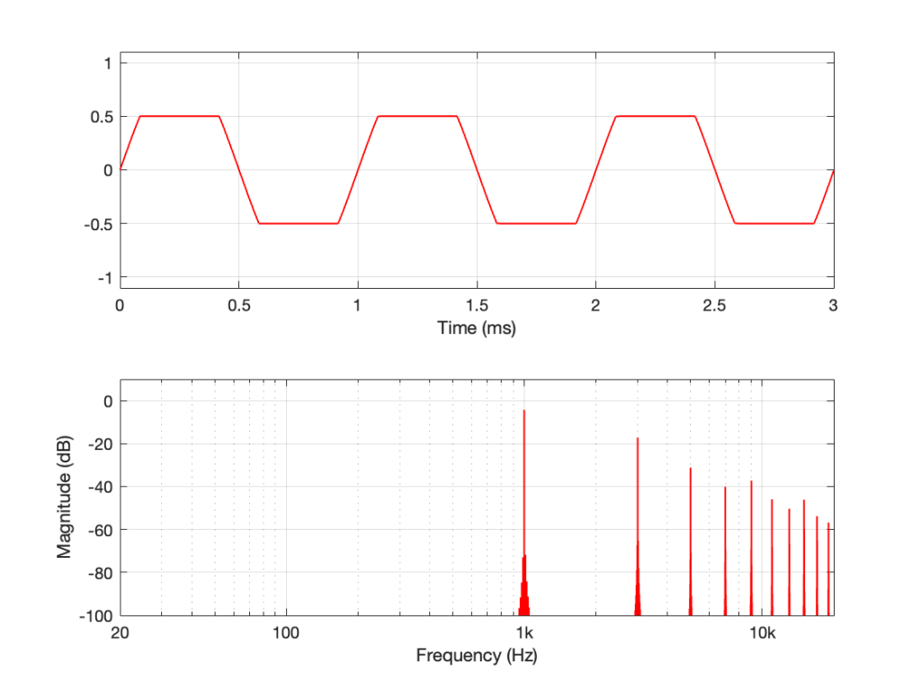
Now, to be fair, what I’m REALLY doing here is to look for the peak value of the measurement signal coming into the DUT, and then clipping it. This would be equivalent to doing a measurement of the DUT and adjusting the input gain so that it looks like a peak level of – 6 dB relative to maximum is coming in.
Also, because what I’m about to do through this series is going to have radical effects on the level after processing, I’m normalising the levels. So, some things won’t look right from a perspective of how-loud-it-appears-to-be.
If I measure that DUT using the three methods, the results look like this:
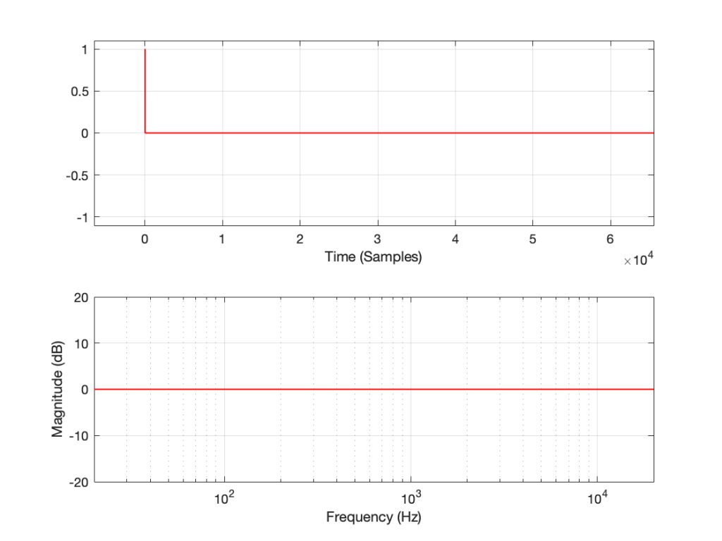
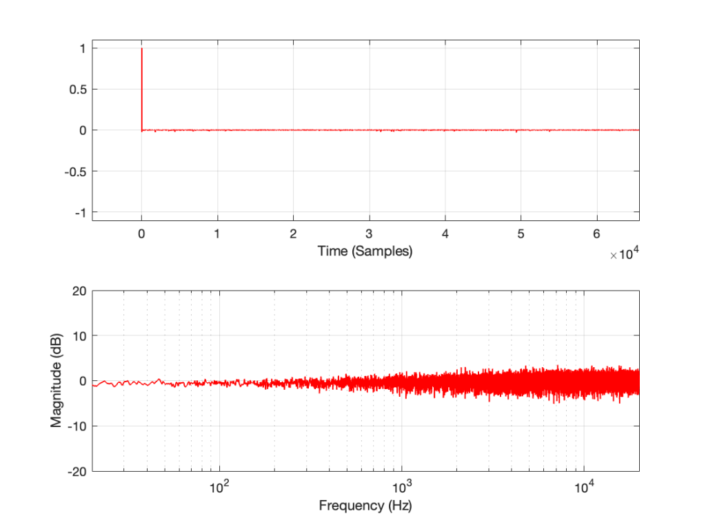
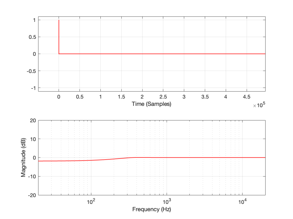
As can easily be seen above, the three systems show very different responses. So, unlike what I claimed this post (which is admittedly over-simplified, although intentionally so to make a point…), the fact that they are measuring the impulse response does not mean that we can’t see the effects of the non-linear response. We can obviously see artefacts in the linear response that are caused by the distortion, but those artefacts don’t look like distortion, and they don’t really show us the real linear response.