In a previous posting, I showed some plots that displayed the probability density functions (or PDF) of a number of commercial audio recordings. (If you are new to the concept of a probability density function, then you might want to at least have a look at that posting before reading further…)

I’ve been doing a little more work on this subject, with some possible implications on how to interpret those plots. Or, perhaps more specifically, with some possible implications on possible conclusions to be drawn from those plots.

 

 

Full-band examples

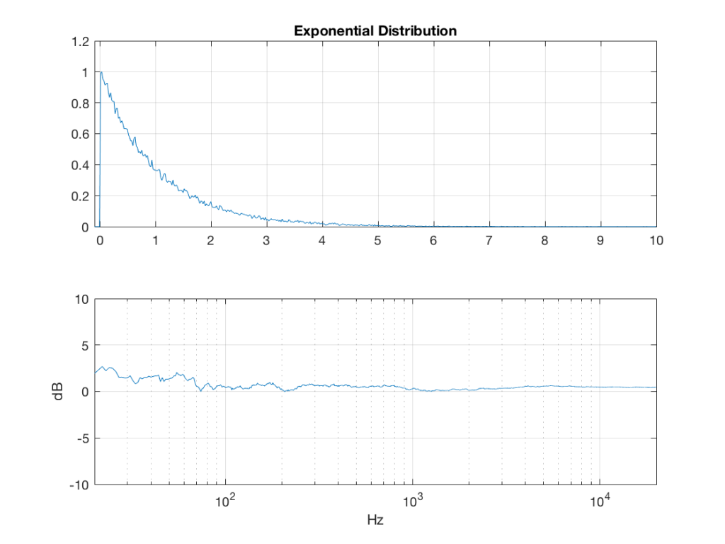
To start, let’s create some noise with a desired PDF, without imposing any frequency limitations on the signal.

To do this, I’ve ported equations from “Computer Music: Synthesis, Composition, and Performance” by Charles Dodge and Thomas A. Jerse, Schirmer Books, New York (1985) to Matlab. That code is shown below in italics, in case you might want to use it. (No promises are made regarding the code quality… However, I will say that I’ve written the code to be easily understandable, rather than efficient – so don’t make fun of me.) I’ve made the length of the noise samples 2^16 because I like that number. (Actually, it’s for other reasons involving plotting the results of an FFT, and my own laziness regarding frequency scaling – but that’s my business.)

 

Uniform (aka Rectangular) Distribution

uniform = rand(2^16, 1);

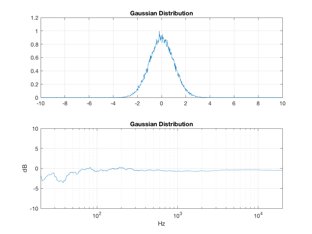
Of course, as you can see in the plots in Figure 1, the signal is not “perfectly” rectangular, nor is it “perfectly” flat. This is because it’s noise. If I ran exactly the same code again, the result would be different, but also neither perfectly rectangular nor flat. Of course, if I ran the code repeatedly, and averaged the results,  the average would become “better” and “better”.

 

Linear Distribution

linear_temp_1 = rand(2^16, 1);

linear_temp_2  = rand(2^16, 1);

temp_indices = find(linear_temp_1 < linear_temp_2);

linear = linear_temp_2;

linear(temp_indices) = linear_temp_1(temp_indices);

 

 

 

Triangular Distribution

triangular = rand(2^16, 1) – rand(2^16, 1);

 

 

Exponential Distribution

lambda = 1;     % lambda must be greater than 0

exponential_temp = rand(2^16, 1) / lambda;

if any(exponential_temp == 0)    % ensure that no values of exponential_temp are 0

    error(‘Please try again…’)

end

exponential = -log(exponential_temp);

 

 

 

Bilateral Exponential Distribution (aka Laplacian)

lambda = 1;     % must be greater than 0

bilex_temp = 2 * rand(2^16, 1);

% check that no values of bilex_temp are 0 or 2

if any(bilex_temp == 0)

    error(‘Please try again…’)

end

bilex_lessthan1 = find(bilex_temp <= 1);

bilex(bilex_lessthan1, 1) = log(bilex_temp(bilex_lessthan1)) / lambda;

bilex_greaterthan1 = find(bilex_temp > 1);

bilex_temp(bilex_greaterthan1) = 2 – bilex_temp(bilex_greaterthan1);

bilex(bilex_greaterthan1, 1) = -log(bilex_temp(bilex_greaterthan1)) / lambda;

 

 

 

Gaussian

sigma = 1;

xmu = 0;   % offset

n = 100; % number of random number vectors used to create final vector (more is better)

xnover = n/2;

sc = 1/sqrt(n/12);

total = sum(rand(2^16, n), 2);

gaussian = sigma * sc * (total – xnover) + xmu; 

 

 

Of course, if you are using Matlab, there is an easier way to get a noise signal with a Gaussian PDF, and that is to use the randn() function.

 

The effects of band-passing the signals

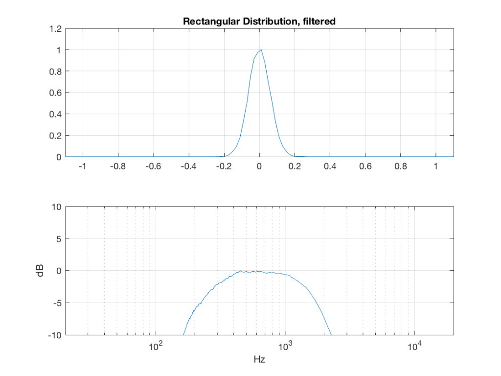
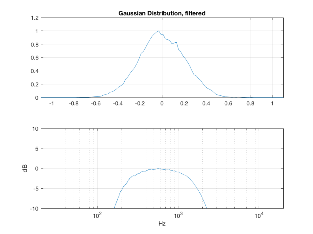
What happens to the probability distribution of the signals if we band-limit them? For example, let’s take the signals that were plotted above, and put them through two sets of two second-order Butterworth filters in series, one set producing a high-pass filter at 200 Hz and the other resulting in a low-pass filter at 2 kHz .(This is the same as if we were making a mid-range signal in a 4th-order Linkwitz-Riley crossover, assuming that our midrange drivers had flat magnitude responses far beyond our crossover frequencies, and therefore required no correction in the crossover…)

What happens to our PDF’s as a result of the band limiting? Let’s see…

 

 

 

 

 

 

 

So, what we can see in Figures 7 through 12 (inclusive) is that, regardless of the original PDF of the signal, if you band-limit it, the result has a Gaussian distribution.

And yes, I tried other bandwidths and filter slopes. The result, generally speaking, is the same.

One part of this effect is a little obvious. The high-pass filter (in this case, at 200 Hz) removes the DC component, which makes all of the PDF’s symmetrical around the 0 line.

However, the “punch line” is that, regardless of the distribution of the signal coming into your system (and that can be quite different from song to song as I showed in this posting) the PDF of the signal after band-limiting (say, being sent to your loudspeaker drivers) will be Gaussian-ish.

 

And, before you ask, “what if you had only put in a high-pass or a low-pass filter?” – that answer is coming in a later posting…

 

Post-script

This posting has a Part 1 that you’ll find here, and a Part 3 that you’ll find here.