A two-part excellent podcast on the effects of sound on our health.

A two-part excellent podcast on the effects of sound on our health.
I love two of the quotes in this nice obituary at Stereophile:
‘… some things that look gross in the frequency response, the ear says, “I don’t care”.’
– Siegfried Linkwitz
“Measurements are useful tools, but don’t let them hold you hostage.”
– Michael Fremer


This “series” of postings was intended to describe some of the errors that I commonly see when I measure and evaluate digital audio systems. All of the examples I’ve shown are taken from measurements of commercially-available hardware and software – they’re not “beta” versions that are in development.
There are some reasons why I wrote this series that I’d like to make reasonably explicit.
Unfortunately, the only thing that I have concluded after having done lots of measurements of lots of systems is that, unless you do a full set of measurements on a given system, you don’t really know how it behaves. And, it might not behave the same tomorrow because something in the chain might have had a software update overnight.
However, there are two more thing that I’d like to point out (which I’ve already mentioned in one of the postings).
Firstly, just because a system has a digital input (or source, say, a file) and a digital output does not guarantee that it’s perfect. These days the weakest links in a digital audio signal path are typically in the signal processing software or the clocking of the devices in the audio chain.
Secondly, if you do have a digital audio system or device, and something sounds weird, there’s probably no need to look for the most complicated solution to the problem. Typically, the problem is in a poor implementation of an algorithm somewhere in the system. In other words, there’s no point in arguing over whether your DAC has a 120 dB or a 123 dB SNR if you have a sampling rate converter upstream that is generating aliasing at -60 dB… Don’t spend money “upgrading” your mains cables if your real problem is that audio samples are being left out every half second because your source and your receiver can’t agree on how fast their clocks should run.
So, the bad news is that trying to keep track of all of this is complicated at best. More likely impossible.
On the other hand, if you do have a system that you’re happy with, it’s best to not read anything I wrote and just keep listening to your music…
As a setup for this posting, I have to start with some background information…
Back when I was doing my bachelor’s of music degree, I used to make some pocket money playing background music for things like wedding receptions. One of the good things about playing such a gig was that, for the most part, no one is listening to you… You’re just filling in as part of the background noise. So, as the evening went on, and I grew more and more tired, I would change to simpler and simpler arrangements of the tunes. Leaving some notes out meant I didn’t have to think as quickly, and, since no one was really listening, I could get away with it.
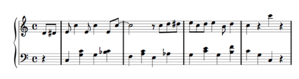
If you watch the short video above, you’ll hear the same composition played 3 times (the 4th is just a copy of the first, for comparison). The first arrangement contains a total of 71 notes, as shown below.

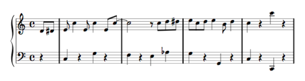
The second arrangement uses only 38 notes, as you can see in Figure 2, below.
The third arrangement uses even fewer notes – a total of only 27 notes, shown in Figure 3, below.
The point of this story is that, in all three arrangements, the piece of music is easily recognisable. And, if it’s late in the night and you’ve had too much to drink at the wedding reception, I’d probably get away with not playing the full arrangement without you even noticing the difference…
A psychoacoustic CODEC (Compression DECompression) algorithm works in a very similar way. I’ll explain…
If you do an “audiometry test”, you’ll be put in a very, very quiet room and given a pair of headphones and a button. in an adjacent room is a person who sees a light when you press the button and controls a tone generator. You’ll be told that you’ll hear a tone in one ear from the headphones, and when you do, you should push the button. When you do this, the tone will get quieter, and you’ll push the button again. This will happen over and over until you can’t hear the tone. This is repeated in your two ears at different frequencies (and, of course, the whole thing is randomised so that you can’t predict a response…)
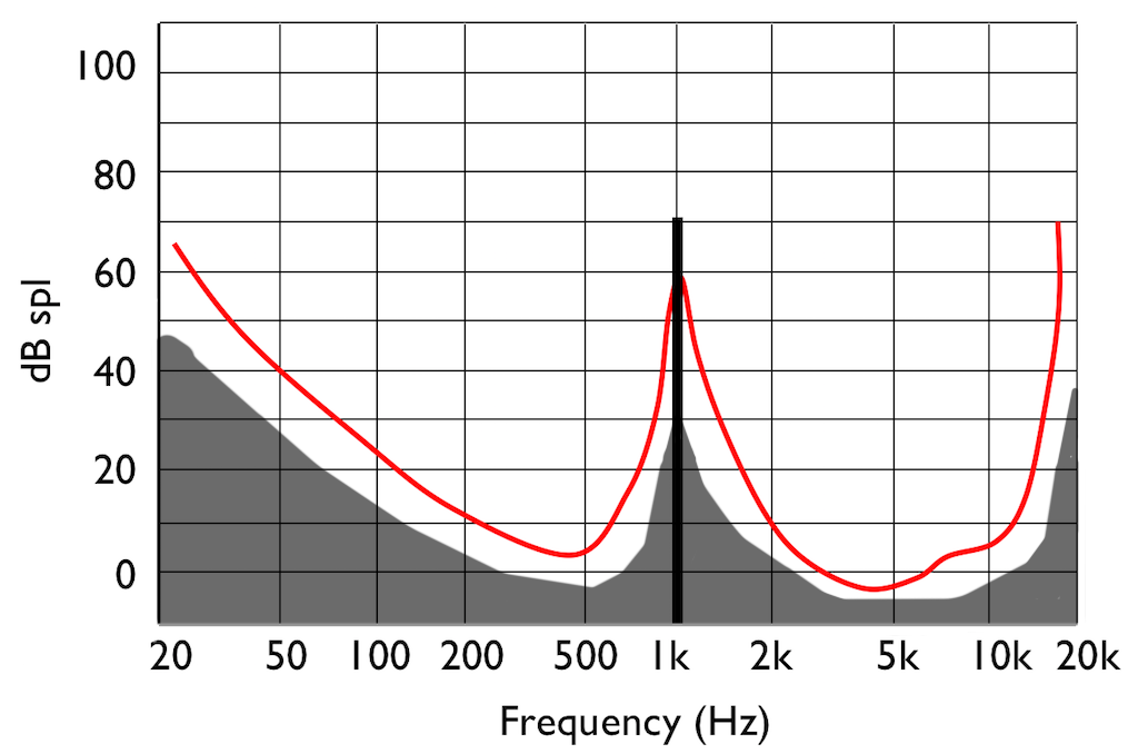
If you do this test, and if you have textbook-quality hearing, then you’ll find out that your threshold of hearing is different at different frequencies. In fact, a plot of the quietest tones you can hear at different frequencies it will look something like that shown in Figure 4.
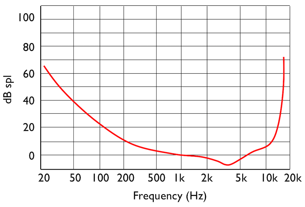
This red curve shows a typical curve for a threshold of hearing. Any frequency that was played at a level that would be below this red curve would not be audible. Note that the threshold is very different at different frequencies.

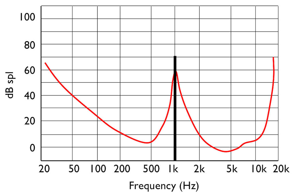
Interestingly, if you do play this tone shown in Figure 5, then your threshold of hearing will change, as is shown in Figure 6.
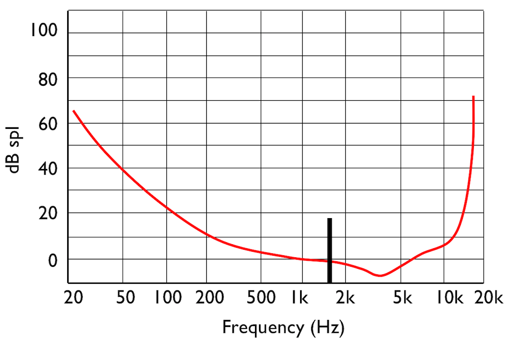
IF you were not playing that loud 1 kHz tone, and, instead, you played a quieter tone just below 2 kHz, it would also be audible, since it’s also above the threshold of hearing (shown in Figure 7.
However, if you play those two tones simultaneously, what happens?
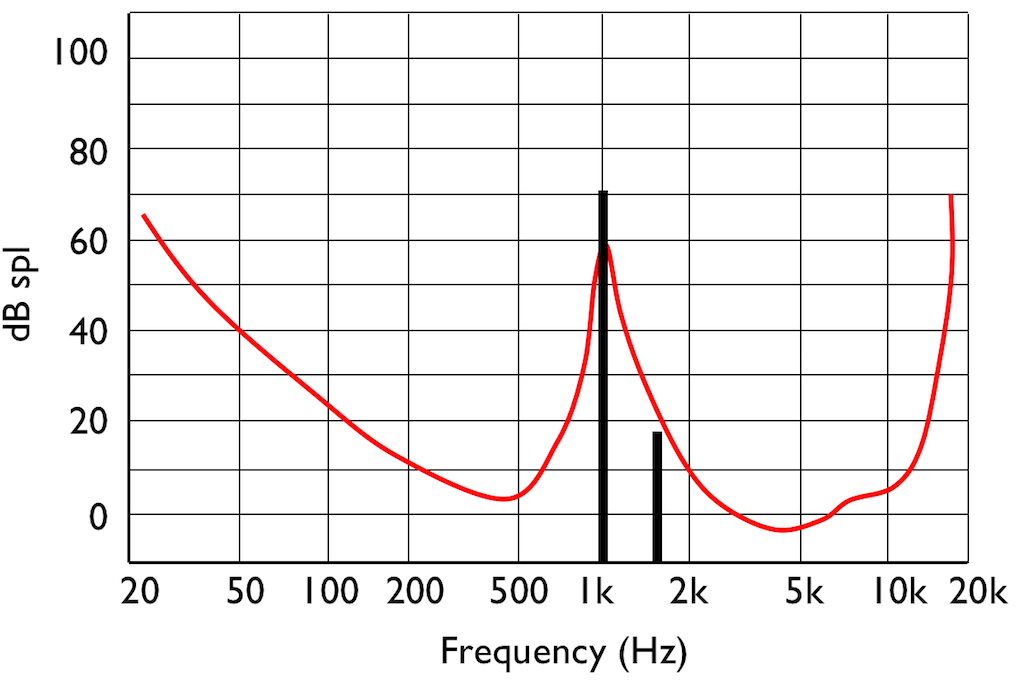
This effect is called “psychoacoustic masking” – the quieter tone is masked by the louder tone if the two area reasonably close together in frequency. This is essentially the same reason that you can’t hear someone whispering to you at an AC/DC concert… Normal people call it being “drowned out” by the guitar solo. Scientists will call it “psychoacoustic masking”.
Let’s pull these two stories together… The reason I started leaving notes out when I was playing background music was that my processing power was getting limited (because I was getting tired) and the people listening weren’t able to tell the difference. This is how I got away with it. Of course, if you were listening, you would have noticed – but that’s just a chance I had to take.
If you want to record, store, or transmit an audio signal and you don’t have enough processing power, storage area, or bandwidth, you need to leave stuff out. There are lots of strategies for doing this – but one of them is to get a computer to analyse the frequency content of the signal and try to predict what components of the signal will be psychoacoustically masked and leave those components out. So, essentially, just like I was trying to predict which notes you wouldn’t miss, a computer is trying to predict what you won’t be able to hear…
This process is a general description of what is done in all the psychoacoustic CODECs like MP3, Ogg Vorbis, AC-3, AAC, SBC, and so on and so on. These are all called “lossy” CODECs because some components of the audio signal are lost in the encoding process. Of course, these CODECs have different perceived qualities because they all have different prediction algorithms, and some are better at predicting what you can’t hear than others. Also, depending on what bitrate is available, the algorithms may be more or less aggressive in making their decisions about your abilities.
There’s just one small problem… If you remove some components of the audio signal, then you create an error, and the creation of that error generates noise. However, the algorithm has an trick up its sleeve. It knows the error it has created, it knows the frequency content of the signal that it’s keeping (and therefore it knows the resulting elevated masking threshold). So it uses that “knowledge” to shape the frequency spectrum of the error to sit under the resulting threshold of hearing, as shown by the gray area in Figure 9.
Let’s assume that this system works. (In fact, some of the algorithms work very well, if you consider how much data is being eliminated… There’s no need to be snobbish…)
Okay – everything above was just the “setup” for this posting.
For this test, I put two .wav files on a NAS drive. Both files had a sampling rate of 48 kHz, one file was a 16-bit file and the other was a 24-bit file.
On the NAS drive, I have two different applications that act as audio servers. These two applications come from two different companies, and each one has an associated “player” app that I’ve put on my phone. However, the app on the phone is really just acting as a remote control in this case.
The two audio server applications on the NAS drive are able to stream via my 2.4 GHz WiFi to an audio device acting as a receiver. I captured the output from that receiver playing the two files using the two server applications. (therefore there were 4 tests run)
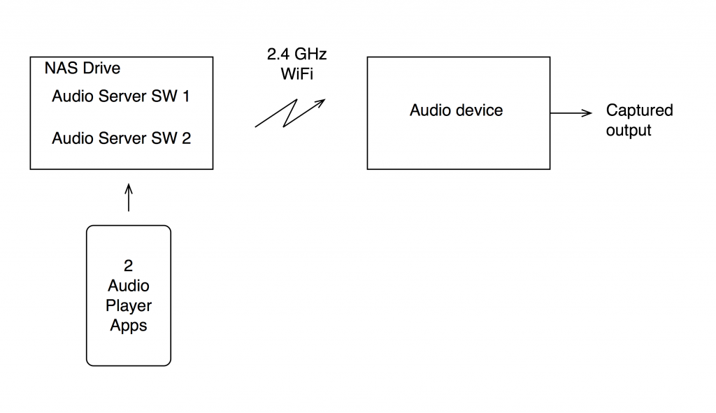
The content of the signal in the two .wav files was a swept sine tone, going from 20 Hz to 90% of Nyquist, at 0 dB FS. I captured the output of the audio device in Figure 10 and ran a spectrogram of the result, analysing the signal down to 100 dB below the signal’s level. The results are shown below.
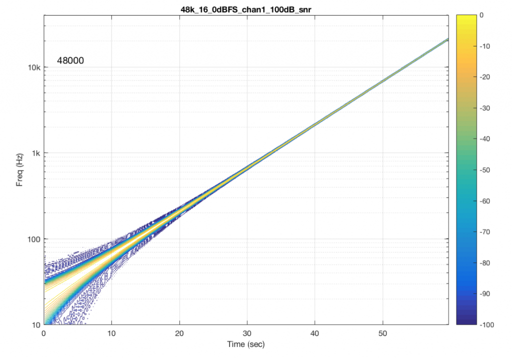


So, Figures 11 and 13 show the same file (the 16-bit version) played to the same output device over the same network, using two different audio server applications on my NAS drive.
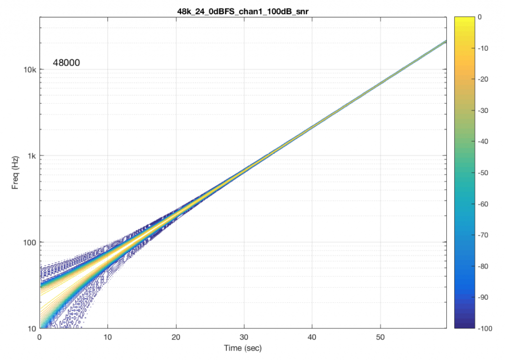
Figures 12 and 14 also show the same file (the 24-bit version). As is immediately obvious, the “Audio Server SW 2” is not nearly as happy about playing the 24-bit file. There is harmonic distortion (the diagonal lines parallel with the signal), probably caused by clipping. This also generates aliasing, as we saw in a previous posting.
However, there is also a lot of visible noise around the signal – the “fuzzy blobs” that surround the signal. This has the same appearance as what you would see from the output of a psychoacoustic CODEC – it’s the noise that the encoder tries to “fit under” the signal, as shown in Figure 9… One give-away that this is probably the case is that the vertical width (the frequency spread) of that noise appears to be much wider when the signal is a low-frequency. This is because this plot has a logarithmic frequency scale, but a CODEC encoder “thinks” on a linear frequency scale. So, frequency bands of equal widths on a linear scale will appear to be wider in the low end on a log scale. (Another way to think of this is that there are as many “Hertz’s” from 0 Hz to 10 kHz as there are from 10 kHz to 20 kHz. The width of both of these bands is 10000 Hz. However, those of us who are still young enough to hear up there will only hear the second of these as the top octave – and there are lots of octaves in the first one. (I know, if we go all the way to 0 Hz, then there are an infinite number of octaves, but I don’t want to discuss Zeno today…))
So, it appears that “Audio Server SW 2” on my NAS drive doesn’t like sending 24 bits directly to my audio device. Instead, it probably decodes the wav file, and transcodes the lossless LPCM format into a lossy CODEC (clipping the signal in the process) and sends that instead. So, by playing a “high resolution” audio file using that application, I get poorer quality at the output.
As always, I’m not going to discuss whether this effect is audible or not. That’s irrelevant, since it’s dependent on too many other factors.
And, as always, I’m not going to put brand or model names on any of the software or hardware tested here. If, for no other reason, this is because this problem may have already been corrected in a firmware update that has come out since I tested it.
The take-home messages here are:
So, if you read a test involving a particular NAS drive, or a particular Audio Server application, or a particular audio device using a file format with a sampling rate and a bit depth and the reviewer says “This system worked perfectly.” You cannot assume that your system will also work perfectly unless all aspects of your system are identical to the tested system. Changing one link in the chain (even upgrading the software version) can wreck everything…
This makes life confusing, unfortunately. However, it does mean that, if someone sounds wrong to you with your own system, there’s no need to chase down excruciating minutiae like how many nanoseconds of jitter you have at your DAC’s input, or whether the cat sleeping on your amplifier is absorbing enough cosmic rays. It could be because your high-res file is getting clipped, aliased, and converted to MP3 before sending to your speakers…
Just in case you’re wondering, I tested these two systems above with all 6 standard sampling rates (44.1, 48, 88.2, 96, 176.4, and 192 kHz), 2 bit depths (16 & 24). I also did two formats (WAV and FLAC) and three signal levels (0, -1, and -60 dB FS) – although that doesn’t matter for this last comment.
“Audio Server SW 2” had the same behaviour in the case of all sampling rates – 16 bit files played without artefacts within 100 dB of the 0 dB FS signal, whereas 24-bit files in all sampling rates exhibited the same errors as are shown in Figure 14.
#79 in a series of articles about the technology behind Bang & Olufsen loudspeakers
“Love at first sight? Let me just put on my glasses.”
Ljupka Cvetanova, The New Land
When I’m working on the sound design for a new pair of (over-ear, closed) headphones, I have to take off my glasses (which makes it difficult for me to see my computer screen…) I’ll explain.
Let’s over-simplify and consider a block diagram of a closed (and therefore “over-ear”) headphone, sitting on one side of your head. This is represented by Figure 1.

One of the important things to note there is that the air in the chamber between the headphone diaphragm and the ear canal is sealed from the outside world.
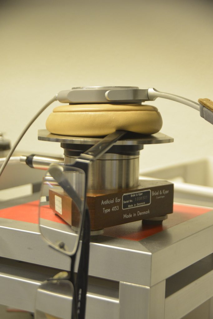
So, if I put such a headphone on an artificial ear (which is a microphone in a small hole in the middle of a plate – it is remarkably well-represented by the red lines in Figure 1….) I can measure its magnitude response. I’ll call this the “reference”. It doesn’t matter to me what the measurement looks like, since this is just a magnitude response which is the combination of the headphone’s response and the artificial ear’s response – with some incorrect positioning thrown into the mix.

If I then remove the headphones from the plate, and put them back on, in what I think is the same position, and then do the measurement again, I’ll get another curve.
Then, I’ll subtract the “reference measurement” (the first one) from the second measurement to see what the difference is. An example of this is plotted in Figure 2.

Now, let’s consider what happens when the seal is broken. I’ll stick a small piece of metal (actually an Allan key, or a hex wrench, depending on where you live) in between the headphones and the plate, causing a leak in the air between the internal cavity and the outside world, as shown in Figure 4.


We then repeat the measurement, and subtract the original Reference measurement to see what happened. This is shown in Figure 6.
As you can see, the leak in the system causes us to lose bass, primarily. In the very low end, the loss is significant – more than 10 dB down at 20 Hz! Basically, what we’ve done here is to create an acoustical high-pass filter. (I’m not going to go into the physics of why this happens… That’s too much information for this posting.) You can also see that there’s a bump around 200 Hz which is also a result of the leak. The sharp peak up at 8 kHz is not caused by the leak – it’s just an artefact of the headphones having moved a little on the plate when I put in the Allen Key.
Now let’s make the leak bigger. I’ll stick the arm of my glasses in between the plate and the leather pad.
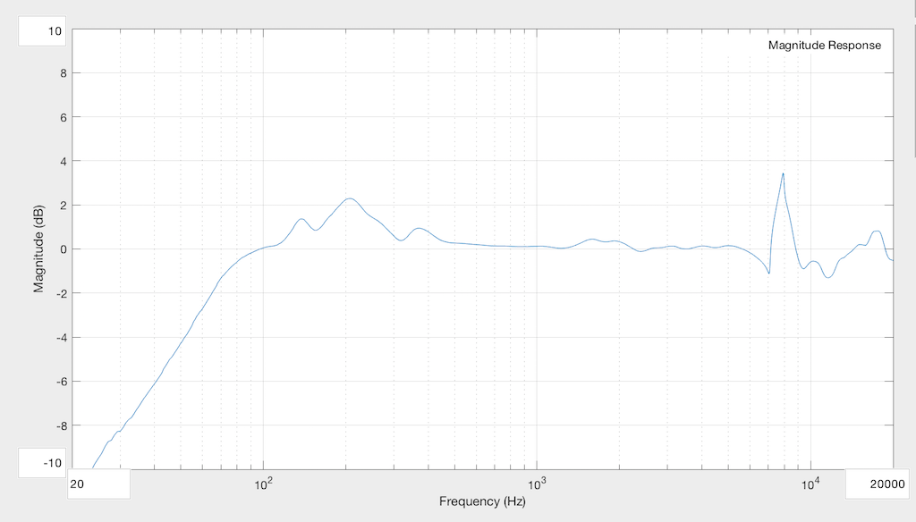
The result of this measurement (again with the Reference subtracted) is shown in Figure 8.

Now you can see that the high pass filter’s cutoff frequency has risen, and the resonance in the system has not only increased in frequency (to 400 Hz or so) but also in magnitude (to almost +10 dB! Again, the sharp wiggles at the top are mostly just artefacts caused by changes in position…
Just to check and see that I haven’t done something stupid, I’ll remove the glasses, and run the measurement again…

The result of this measurement is shown in Figure 10.

So, there are a couple of things to be learned here…
Firstly, if you and a friend both listen to the same pair of closed, sealed headphones, and you disagree about the relative level of bass, check that you’re both not wearing glasses or large earrings…
The more general interpretation of that previous point is that small leaks in the system have a big effect on the response of the headphones in the low-frequency region. Those leaks can happen as a result of many things – not just the arm of your glasses. Hair can also cause the problem. Or, for example, if the headphones are slightly big, and/or your head is slightly small, then the area where your jaw meets your neck under your pinna (around your mastoid gland) is one possile place for leaks. This can also happen if you have a very sharp corner around your jaw (say you are Audrey Hepburn, for example), and the ear cup padding is stiff. Interestingly, as time passes, the foam and covering soften and may change shape slightly to seal these leaks. So, as the headphones match the shape of your head over time, you might get a better seal and a change in the bass level. This might be interpreted by some people as having “broken in” the headphones – but what you’ve actually done is to “break in” the padding so that it fits your head better.
Secondly, those big, sharp spikes up the high end aren’t insignificant… They’re the result of small movements in the headphones on the measuring system. A similar thing happens when you move headphones on your head – but it can be even more significant due to effects caused by your pinna. This is why, many people, when doing headphone measurements, will do many measurements (say, 5 to 10) and average the results. Those errors in placement are not just the result of shifts on the plate – they may also be caused by differences in “clamping pressure” – so, if I angled the headphones a little on that table, then they might be pressing harder on the artificial ear, possibly only on one side of the ear cup, and this will also change the measured response in the high frequency bands.

Of course, it’s possible to reduce this problem by making the foam more compliant (a fancy word for “squishy”) – which may, in turn, mean that the response will be more different for different users due to different head widths. Or the problem could be reduced by increasing the clamping force, which will in turn make the headphones uncomfortable because they’re squeezing your head. Or, you could embrace the leak, and make a pair of open headphones – but those will not give you much passive noise isolation from the outside world. In fact, you won’t have any at all…
So as you can see, as a manufacturer, this issue has to be balanced with other issues when designing the headphones in the first place…
Or you can just take off your glasses, close your eyes, and listen…
Please don’t jump too far in your conclusions as a result of seeing these measurements. You should NOT interpret them to mean that, if you wear glasses, you will get a 10 dB bump at 400 Hz. The actual response that you will get from your headphones depends on the size of the leak, the volume of the chamber in the ear cup (which is partly dependent on the size of your pinna, since that occupies a significant portion of the volume inside the chamber) and other factors.
The take-home message here is: when you’re evaluating a pair of closed, over-ear headphones: small leaks have an effect on the low frequency response, and small changes in position have an effect on the high-frequency response. The details of those effects are almost impossible to predict accurately.