The June, 1968 issue of Wireless World magazine includes an article by R.T. Lovelock called “Loudness Control for a Stereo System”. This article partly addresses the issue of resistance behaviour one or more channels of a variable resistor. However, it also includes the following statement:
It is well known that the sensitivity of the ear does not vary in a linear manner over the whole of the frequency range. The difference in levels between the threshold of audibility and that of pain is much less at very low and very high frequencies than it is in the middle of the audio spectrum. If the frequency response is adjusted to sound correct when the reproduction level is high, it will sound thin and attenuated when the level is turned down to a soft effect. Since some people desire a high level, while others cannot endure it, if the response is maintained constant while the level is altered, the reproduction will be correct at only one of the many preferred levels. If quality is to be maintained at all levels it will be necessary to readjust the tone controls for each setting of the gain control
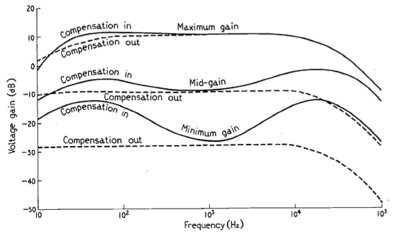
The article includes a circuit diagram that can be used to introduce a low- and high-frequency boost at lower settings of the volume control, with the following example responses:
These days, almost all audio devices include some version of this kind of variable magnitude response, dependent on volume. However, in 1968, this was a rather new idea that generated some debate.
In the following month’s issue The Letters to the Editor include a rather angry letter from John Crabbe (Editor of Hi-Fi News) where he says
Mr. Lovelock’s article in your June issue raises an old bogey which I naively thought had been buried by most British engineers many years ago. I refer, not to the author’s excellent and useful thesis on achieving an accurate gain control law, but to the notion that our hearing system’s non-linear loudness / frequency behaviour justifies an interference with response when reproducing music at various levels.
Of course, we all know about Fletcher-Munson and Robinson-Dadson, etc, and it is true that l.f. acuity declines with falling sound pressure level; though the h.f. end is different, and latest research does not support a general rise in output of the sort given by Mr. Lovelock’s circuit. However, the point is that applying the inverse of these curves to sound reproduction is completely fallacious, because the hearing mechanism works the way it does in real life, with music loud or quiet, and no one objects. If `live’ music is heard quietly from a distant seat in the concert hall the bass is subjectively less full than if heard loudly from the front row of the stalls. All a `loudness control’ does is to offer the possibility of a distant loudness coupled with a close tonal balance; no doubt an interesting experiment in psycho-acoustics, but nothing to do with realistic reproduction.
In my experience the reaction of most serious music listeners to the unnaturally thick-textured sound (for its loudness) offered at low levels by an amplifier fitted with one of these abominations is to switch it out of circuit. No doubt we must manufacture things to cater for the American market, but for goodness sake don’t let readers of Wireless World think that the Editor endorses the total fallacy on which they are based.
with Lovelock replying:
Mr. Crabbe raises a point of perennial controversy in the matter of variation of amplifier response with volume. It was because I was aware of the difference in opinion on this matter that a switch was fitted which allowed a variation of volume without adjustment of frequency characteristic. By a touch of his finger the user may select that condition which he finds most pleasing, and I still think that the question should be settled by subjective pleasure rather than by pure theory.
and
Mr. Crabbe himself admits that when no compensation is coupled to the control, it is in effect a ‘distance’ control. If the listener wishes to transpose himself from the expensive orchestra stalls to the much cheaper gallery, he is, of course, at liberty to do so. The difference in price should indicate which is the preferred choice however.
In the August edition, Crabbe replies, and an R.E. Pickvance joins the debate with a wise observation:
In his article on loudness controls in your June issue Mr. Lovelock mentions the problem of matching the loudness compensation to the actual sound levels generated. Unfortunately the situation is more complex than he suggests. Take, for example, a sound reproduction system with a record player as the signal source: if the compensation is correct for one record, another record with a different value of modulation for the same sound level in the studio will require a different setting of the loudness control in order to recreate that sound level in the listening room. For this reason the tonal balance will vary from one disc to another. Changing the loudspeakers in the system for others with different efficiencies will have the same effect.
In addition, B.S. Methven also joins in to debate the circuit design.
Apart from the fun that I have reading this debate, there are two things that stick out for me that are worth highlighting:
Notice that there is a general agreement that a volume control is, in essence, a distance simulator. This is an old, and very common “philosophy” that we forget these days.
Pickvance’s point is possibly more relevant today than ever. Despite the amount of data that we have with respect to equal loudness contours (aka “Fletcher and Munson curves”) there is still no universal standard in the music industry for mastering levels. Now that more and more tracks are being released in a Dolby Atmos-encoded format, there are some rules to follow. However, these are very different from 2-channel materials, which have no rules at all. Consequently, although we know how to compensate for changes in response in our hearing as a function of level, we don’t know what the reference level should be for any given recording.
The July 1968 issue of Wireless World Magazine contains a description of an early, but interesting analysis of the relationship between phantom image placement in a 2-channel stereo system and interchannel level differences. This is an old favourite topic of mine, originally inspired by the work of Michael Williams and his “Stereophonic Zoom”, and extending to my first AES paper in 1999.
If you, like me, are interested in this (for example, if you’re making a panning algorithm or you’re testing the veracity of headphone-based “virtual” systems), some important figures from that article are shown below.
The typical way of showing the relationship between IAD and phantom image placement.
This one is interesting because it shows the different results in different rooms, (which would also be influenced by loudspeaker directivity.)
Note that, for the plots above and below, the x-axes show the position of the image in the stereo sound stage, where 0 is the centre point between the two loudspeakers and 0.5 is a position in one of the two loudspeakers. This is 0.5 because it’s one-half of the total angular distance between the two loudspeakers. So, you can consider the loudspeaker aperture as ±0.5.
The relationship between image WIDTH and position. This is something I’ve not seen expressed so clearly before.
For more information similar to this, see these links as a start:
In Part 2, I showed the raw magnitude response results of three pairs of headphones measured on three different systems, each done 5 times. However, when you plot magnitude responses on a scale with 80 dB like I did there, it’s difficult to see what’s going on.
Differences in measurements relative to average
One way to get around this issue is to ignore the raw measurement and look at the differences between them, which is what we’ll do here. This allows us to “zoom in” on the variations in the measurements, at the cost of knowing what the general overall responses are.
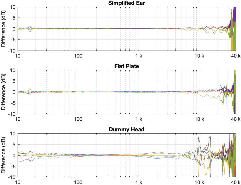
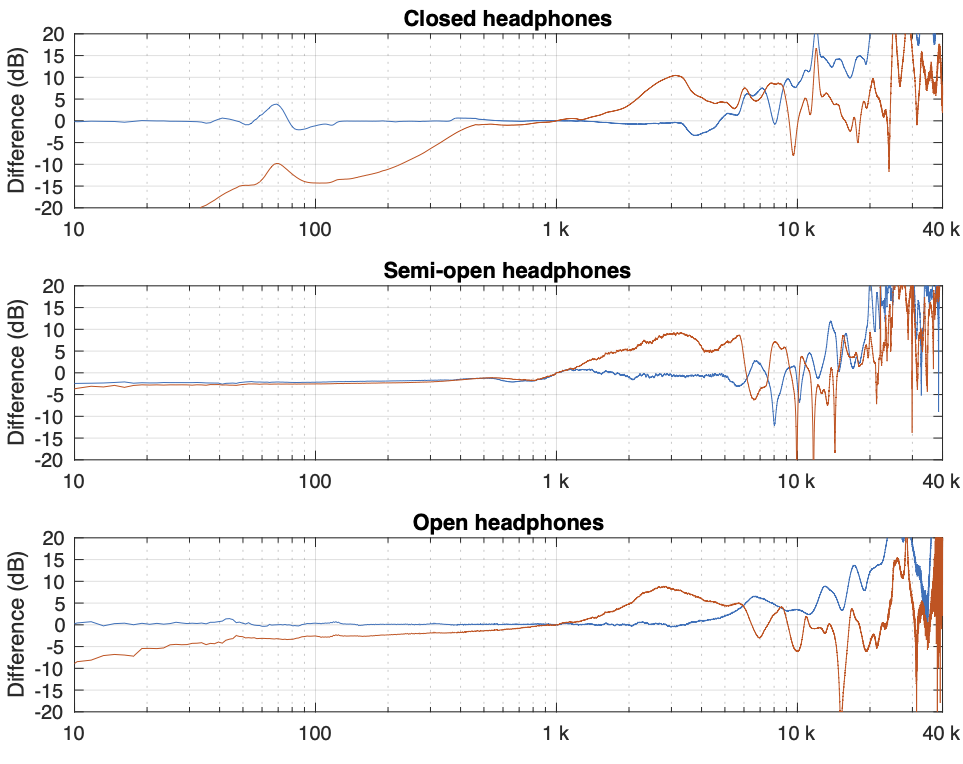
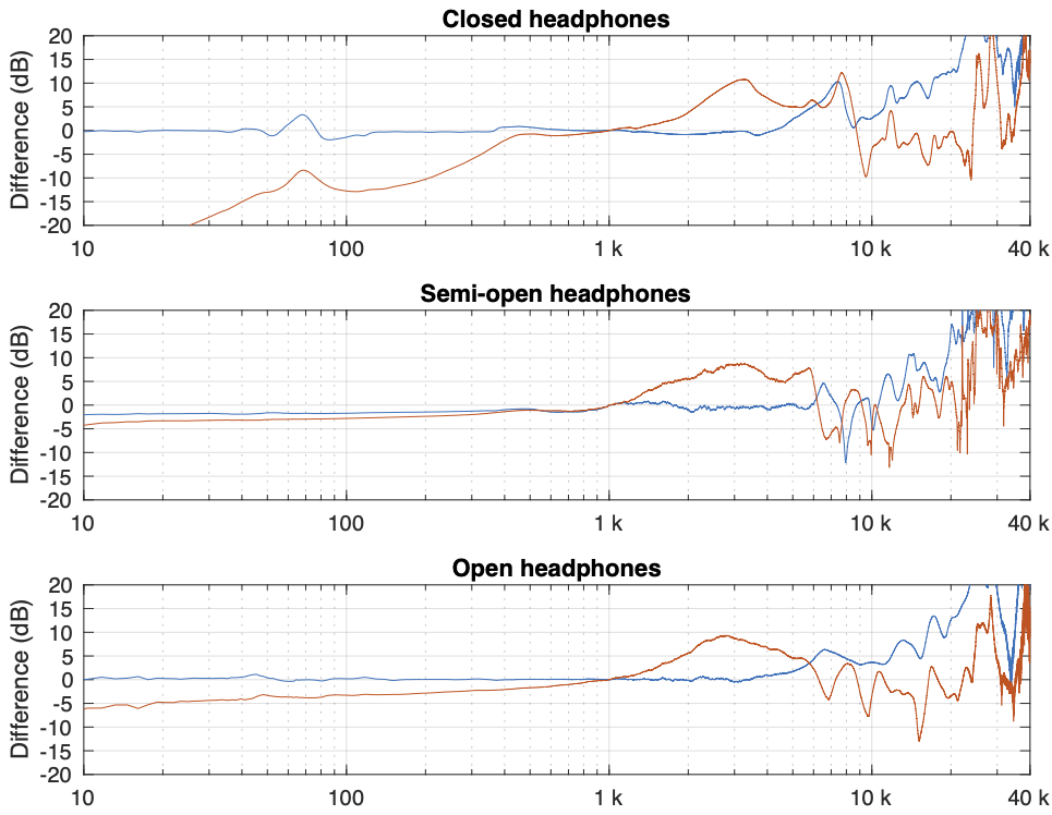
Figure 1 in Part 2 showed the 5 x 3 sets of raw magnitude responses of the open headphones. I then take each set of 5 measurements (remember that these 5 measurements were done by removing the headphones and re-setting them each time on the measurement rig) and find their average response. Then I plot the difference between each of the 5 measurements and that average, and this is done for each of the three measurement systems, as shown below in Figure 1.
Figure 1: Open headphones: The difference between each of the 5 measurements done on each system and the mean (average) of those 5 measurements.
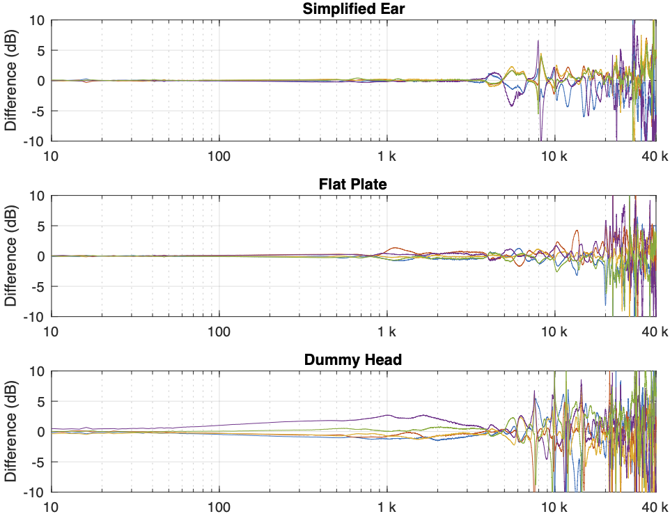
Figure 2: Semi-open headphones: The difference between each of the 5 measurements done on each system and the mean (average) of those 5 measurements.
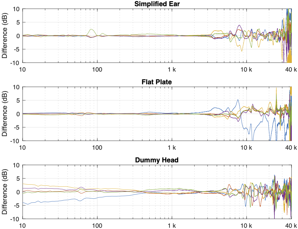
Figure 3: Closed headphones: The difference between each of the 5 measurements done on each system and the mean (average) of those 5 measurements.
Some of the things that were intuitively visible in the plots in Part 2 are now obvious:
There is a huge change in the measured magnitude response in the high frequency bands, even when the pair of headphones and the measurement rig are the same. This is the result of small changes in the physical position of the headphones on the rig, as well as changes in the clamping force (modified by moving the headband extension). I intentionally made both of these “errors” to show the problem. Notice that the differences here are greater than ±10 dB, which is a LOT.
Overall, the differences between the measurements on the dummy head are bigger and have a lower frequency range than for the other two systems. This is mostly due to two things:
because the dummy head has pinnae (ears), very small changes in position result in big changes in response
it is easier to have small leaks around the ear cushions on a dummy head than with a flat surrounding of a metal plate or an artificial ear. This is the reason for the low-frequency differences with the closed headphones. Leaks have no effect on open headphone designs, since they are always leaking out through the diaphragm itself.
The differences that you can see here are the reason that, when we’re measuring headphones, we never measure just once. We always do a minimum of 5 measurements and look at the average of the set. This is standard practice, both for headphone developers and experienced reviewers like this one, for example.
In addition to this averaging, it’s also smart to do some kind of smoothing (which I have not done here…) to avoid being distracted by sharp changes in the response. Sharp peaks and dips can be a problem, particularly when you look at the phase response, the group delay, or looking for ringing in the time domain. However, it’s important to remember that the peaks and dips that you see in the measurements above might not actually be there when you put the headphones on your head. For example, if the variations are caused by standing waves inside the headphones due to the fact that the measurement system itself is made of reflective plastic or metal (but remember that you aren’t…) then the measurement is correct, but it doesn’t reflect (ha ha…) reality…
One additional thing to remember with these plots is that something that looks like a peak in the curve MIGHT be a peak, but it might also be a dip in the average curve because we’re only looking at the differences in the responses.
System differences
Instead of looking at the differences between each individual measurement and the average of the measurement set, we can also look at the differences between what each measurement system is telling us for each headphone type. For example, if I take one measurement of a pair of headphones on each system, and pretend that one of them is “correct”, then I can find the difference between the measurements from the other two systems and that “reference”.
Figure 4. One measurement for each pair of headphones on each measurement system. The red curves are the dummy head and the blue curves are the artificial ear RELATIVE TO THE FLAT PLATE.
In Figure 4, I’m pretending that the flat plate is the “correct” system, and then I’m plotting the difference between the dummy head measurement (in red) and the artificial ear measurement (in blue) relative to it.
Again, it’s important to remember with these plots is that something that looks like a peak in the curve might actually be a dip in the “reference” curve. (The bump in the red lines around 2 – 3 kHz is an example of this…)
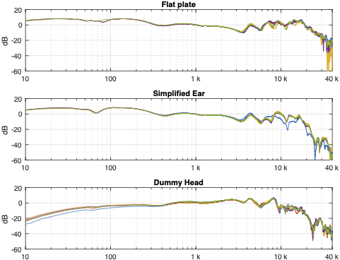
Of course, you could say “but you just said that we shouldn’t look at a single measurement”… which is correct. If we use the averages of all 5 measurements for each set and do the same plot, the result is Figure 5.
Figure 5. The average of all 5 measurements for each pair of headphones on each measurement system. The red curves are the dummy head and the blue curves are the artificial ear relative to the flat plate.
You can see there that, by using the averaged responses instead of individual measurements, the really sharp peaks and dips disappear, since they smooth each other out.
Comparing headphone types
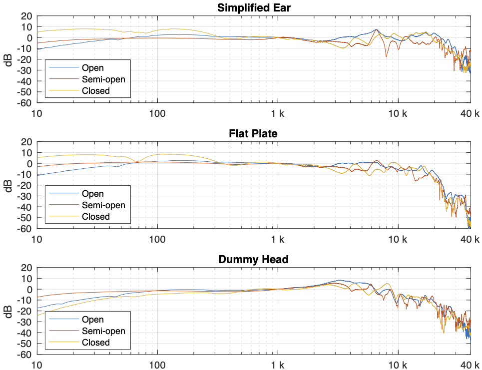
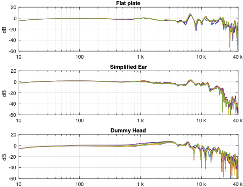
Things get even more complicated if you try to compare the headphones to each other using the measurement systems. Figure 6, below, shows the averages of the five measurements of each pair of headphones on each measurement system, plotted together on the same graphs (normalised to the levels at 1 kHz), one for each measurement system.
Figure 6: Comparing the three pairs of headphones on each measurement system.
This is actually a really important figure, since it shows that the same headphones measured the same way on different systems tell you very different things. For example, if you use the “simplified ear” or the “flat plate” system, you’ll believe that the closed headphones (the yellow line) is about 10 – 15 dB higher than the open headphones (the blue line) in the low frequency region. However, if you use the “dummy head” system, you’ll believe that the closed headphones (the yellow line) is about 5 – 10 dB lower than the open headphones (the blue line) in the low frequency region.
Which one is correct? They all are, even though they tell you different things. After all, it’s just data… The reason this happens is that one measurement system cannot be used to directly compare two different types of headphones because their acoustic impedances are different. With experience, you can learn to interpret the data you’re shown to get some idea of what’s going on. However, “experience” in that sentence means “years of correlating how the headphones sound with how the plots look with the measurement system(s) you use”. If you aren’t familiar with the measurement system and how it filters the measurement, then you won’t be able to interpret the data you get from it.
That said, you MIGHT be able to use one system to compare two different pairs of open headphones or two different pairs of closed headphones, but you can’t directly compare measurements of different headphone types (e.g. open and closed) reliably.
This also means that, if you subscribe to two different headphone magazines both of which use measurements as part of their reviews, and one of them uses a flat plate system while the other uses a dummy head, the same pairs of headphones might get opposite reviews in the two magazines…
Which review can you trust? Both of them – and neither of them.
Conclusions
Looking at these plots, you could come to the conclusion that you can’t trust anything, because no two measurements tell you the same things about the same devices. This is the incorrect conclusion to draw. These measurement systems are tools that we use to tell us something about the headphones on which we’re working. And people who use these tools daily know how to interpret the data they see from them. If something looks weird, they either expected it to look weird, or they run the measurement on another system to get a different view.
The danger comes when you make one measurement on one device and hold that up as The Truth. A result that you get from any one of these systems is not The Truth, but it is A Truth – you just need more information. If you’re only shown one measurement (or even an average of measurements) that was done on only one measurement system, then you should raise at least one eyebrow, and ask some questions about how that choice of system affects the plots that you see.
In many ways, it’s like looking at a recipe in a cookbook. You might be able to determine whether you might like or probably hate a dish by reading its description of ingredients and how to prepare it. But you cannot know how it’ll taste until you make it and put it in your mouth. And, if you cook like I do, it’ll be just a little different next time. It’s cooking – not a chemistry experiment. If you use headphones like I do, it’ll also be a little different next time because some days, I don’t wear my glasses, or I position the head band a little differently, so the leak around the ear cushion or the clamping force is a little different.
In Part 1, I talked about how any measurement of an audio device tells you something about how it behaves, but you need to know a LOT more than what you can learn from one measurements. This is especially true for a loudspeaker where you have the extra dimensions of physical space to consider.
Thought experiment: Fridges vs. Mosquitos
Consider a situation where you’re sitting at your kitchen table, and you can hear the compressor in your fridge humming/buzzing over on the other side of the room. If you make a small movement in your chair, the hum from the fridge sounds the same to you. This is partly because the distance from the fridge to you is much bigger than the changes in that distance that result from you shifting your butt.
Now think about the times you’ve been trying to sleep on a summer night, and there’s a mosquito that is flying near your ear. Very small changes in the location of that mosquito result in VERY big changes in how it sounds to you. This is because, relative to the distance to the mosquito, the changes in distance are big.
In other words, in the case of the fridge (that’s say, 3 m away) by moving 10 cm in your chair, you were changing the distance by about 3%, but the mosquito was changing its distance by more than 100% by moving just from 1 cm to 2 cm away.
In other words, a small change in distance makes a big change in sound when the distance is small to begin with.
The challenges of measuring headphones
The methods we use for measuring the magnitude response of a pair of headphones is similar to that used for measuring a loudspeaker. We send a measurement signal to the headphones from a computer, that signal comes out and is received by a microphone that sends its output back to the computer. The computer then is used to determine the difference between what it sent out and what came back. Simple, right?
Wrong.
The problems start with the fact that there are some fundamental differences between headphones and loudspeakers. For starters, there’s no “listening room” with headphones, so we don’t put a microphone 3 m away from the headphones: that wouldn’t make any sense. Instead, we put the headphones on some kind of a device that either simulates an ear, or a head, or a head with ears (with or without ear canals), and that device has a microphone (roughly) where your eardrum would be. Simple, right?
Wrong.
The problem in that sentence was the word “simulates”. How do you simulate an ear or a head or a head with ears? My ears are not shaped identically to yours or anyone else’s. My head is a different size than yours. I don’t have any hair, but you might. I wear glasses, but you might not. There are many things that make us different physically, so how can the device that we use to measure the headphones “simulate” us all? The simple answer to this question is “it can’t.”
This problem is compounded with the fact that measurement devices are usually made out of plastic and metal instead of human skin, so the headphones themselves “see” a different “acoustic load” on the measurement device than they do when they’re on a human head. (The people I work with call this your acoustic impedance.)
However, if your day job is to develop or test headphones, you need to use something to measure how they’re behaving. So, we do.
Headphone measurement systems
There are three basic types of devices that are used to measure headphones.
an artificial ear is typically a metal plate with a depression in the middle. At the bottom of the depression is a microphone. In theory, the acoustic impedance of this is similar to a human ear/pinna + the surrounding part of your head. In practice, this is impossible.
a headphone test fixture looks like a big metal can lying on its side (about the size of an old coffee can, for example) on a base. It might have flat metal sides, or it could have rubber pinnae (the fancy word for ears) mounted on it instead. In the centre of each circular end is a microphone.
a dummy head looks like a simplified model of a human head (typically a man’s head). It might have pinnae, but it might not. If it does, those pinnae might look very much like human ears, or they could look like simplified versions instead. There are microphones where you would expect them, and they might be at the bottom of ear canals, but you can also get dummy heads without ear canals where the microphones are flush with the side of the head.
The test system you use is up to you – but you have to know that they will all tell you something different. This is not only because each of them has a different acoustic response, but also because their different shapes and materials make the headphones themselves behave differently.
That last sentence is important to remember, not just for headphone measurement systems but also for you. If your head and my head are different from each other, AND your pinnae and my pinnae are different from each other, THEN, if I lend you my headphones, the headphones themselves will behave differently on your head than they do on my head. It’s not just our opinions of how they sound that are different – they actually sound different at our two sets of eardrums.
General headphone types
If I oversimplify headphone design, we can talk about two basic acoustical type of headphones: They can be closed (where the back of the diaphragm is enclosed in a sealed cabinet, and so the outside of the headphones is typically made of metal or plastic) or open (where the back of the diaphragm is exposed to the outside world, typically through a metal screen). I’d say that some kinds of headphones can be called semi-open, which just means that the screen has smaller (and/or fewer) holes in it, so there’s less acoustical “transparency” to the outside world.
Examples
To show that all these combinations are different, I took three pairs of headphones
open headphones
semi-open headphones
closed headphones
and I measured each of them on three test devices
artificial “simplified” ear
text fixture with a flat-plate
dummy head
In addition, to illustrate an additional issue (the “mosquito problem”), I did each of these 9 measurements 5 times, removing and replacing the headphones between each measurement. I was intentionally sloppy when placing the headphones on the devices, but kept my accuracy within ±5 mm of the “correct” location. I also changed the clamping force of the headphones on the test devices (by changing the extension of the headband to a random place each time) since this also has a measurable effect on the measured response.
Do not bother asking which headphones I measured or which test systems I used. I’m not telling, since it doesn’t matter. Not to me, anyway…
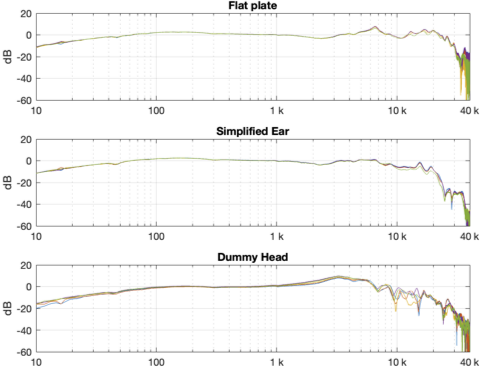
The raw results
I did these measurements using a 10-second sinusoidal sweep from 2 Hz to Nyquist, on a system running at 96 kHz. I’m plotting the magnitude responses with a range from 10 Hz to 40 kHz. However, since the sweep starts at 2 Hz, you can’t really trust the results below 20 Hz (a decade below the lowest frequency of interest is a good rule of thumb when using sine sweeps).
Figure 1: The “raw” magnitude responses of the open headphones measured 5 times each on the three systems
Figure 2: The “raw” magnitude responses of the semi-open headphones measured 5 times each on the three systems
Figure 3: The “raw” magnitude responses of the closed headphones measured 5 times each on the three systems
Looking at the results in the plots above, you can come to some very quick conclusions:
All of the measurements are different from each other, even when you’re looking at the same headphones on the same measurement device. This is especially true in the high frequency bands.
Each pair of headphones looks like it has a different response on each measurement system. For example, looking at Figure 3, the response of the headphones looks different when measured on a flat plate than on a dummy head.
The difference in the results of the systems are different with the different headphone types. For example, the three sets of plots for the “semi-open” headphones (Fig. 2) look more similar to each other than the three sets of plots for the “closed” headphones (Fig. 3)
the scale of these differences is big. Notice that we have an 80 dB scale on all plots… We’re not dealing with subtleties here…
In Part 3 of this series, we’ll dig into those raw results a little to compare and contrast them and talk a little about why they are as different as they are.
People who work in the audio industry use all kinds of different measurements to evaluate the performance of equipment. In many cases, the measurements we do are chosen because they’re easy to do (or because they were easy to do in “The Old Days”), and not because they accurately represent how the equipment actually behaves.
Magnitude response
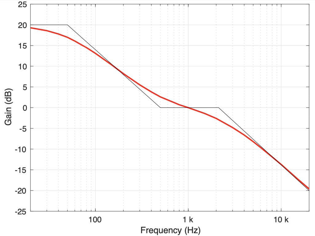
One simple example of this is what most people call a frequency response but what is actually a magnitude response. This is a measure of how the level of an audio signal is changed by the device under test (the “DUT”) as a function of frequency. For example, if you’re measuring a RIAA-spec preamplifier (used for converting a turntable’s pickup’s output to a “line” level signal), then it should have a magnitude response that looks like the red line in the plot in Figure 1.
Figure 1: The red line shows the correct magnitude response for the frequency-dependent filtering in a RIAA phono preamplifier.
This curve shows that, relative to a signal at 1 kHz, the lower the frequency, the more gain is applied to the signal and the higher the frequency, the more attenuation is applied to the signal. Note that this curve is normalised to the level at 1 kHz, which should actually be +40 dB higher if we were to include the frequency-independent gain of the system.
It’s important to remember that this plot shows us only one thing: the change in level caused by the DUT as a function of a change in frequency of the signal. What this plot does NOT show us is much, much more… For example:
We don’t know anything about the behaviour of the system outside the boundaries of this plot.
We don’t know anything about its phase response.
We don’t know anything about how loud the noise of the DUT is.
We don’t know if this plot is true if we were to measure the DUT at a different input level.
We don’t know whether the DUT would have a different behaviour if the device that was feeding it had a different output impedance.
We don’t know whether the DUT would have a different behaviour if the device that it was feeding had a different input impedance.
We don’t know anything about whether the signal has any non-linear distortion artefacts. (Notice that I didn’t say “…whether the signal is distorted” because we know it’s distorted, since the output of the DUT is not the same as the input of the DUT. Any change in the signal is a form of distortion of the signal.)
I’m not saying that a simple magnitude response plot of a DUT is not useful. I’m just saying that it’s not enough information. It’s like asking for the temperature of a cup of coffee. It’s useful information, but it doesn’t tell you enough to know whether you’re going to enjoy drinking it (unless, of course, you hate coffee…)
This problem gets even worse when you’re measuring the acoustic output of a device like a loudspeaker or a pair of headphones, for example. (The acoustic input of a microphone is a similar problem in the opposite direction.)
Let’s start by thinking about a loudspeaker’s output in real life.
You have a device that radiates sound in space in all directions. Let’s look at that space from the loudspeaker’s perspective and say that this means an angle of rotation around the loudspeaker, and an angle of elevation above/below the loudspeaker. That makes two dimensions.
If we’re talking about the loudspeaker’s magnitude response, then we’re looking at its output level (one dimension) as a function of frequency (one more dimension).
That speaker is (usually) in a room, and you’re probably also there too. We can then that this is in three-dimensional space when we talk about the walls, floor, ceiling, and your location inside that space.
Since the surfaces in the room reflect the audio signal, then the time at which the signal arrives at the listening position must also be considered. The “sound” of a loudspeaker at a listening position before the first reflection arrives is different than after a bunch of reflections are coming in and the room has started resonating as well. So, time adds one more dimension to the problem.
We’ll ignore the non-linear distortion artefacts produced by the loudspeaker and the fact that they radiate in different directions differently, since it’s already complicated enough… However, if we were to add things like changes in the response due to temperature of the voice coil or directionally-dependent distortion artefacts like breakup, this would wind up being a much longer discussion…
So, just looking at the small list of “usual suspects” above, we can see that evaluating the sound of a single loudspeaker in a listening room is at least an 8-dimensional problem. And this doesn’t even take things like 2-channel stereo or 7.1.4 multichannel or whether you’re listening to Aretha Franklin or Stockhausen into account…
In other words, it’s complicated. So, we use reductionism to try to start to get an idea of what’s going on. We put a microphone directly in front of a loudspeaker and measure its magnitude response at one level using one kind of test signal (e.g. a swept sine wave or an MLS) and we remove all the room’s reflections somehow. This reduces our 8-dimensional problem to a 2-dimensional version: we have level as a function of frequency and nothing else, since we’ve chosen to throw away everything else by the way we did the measurement.
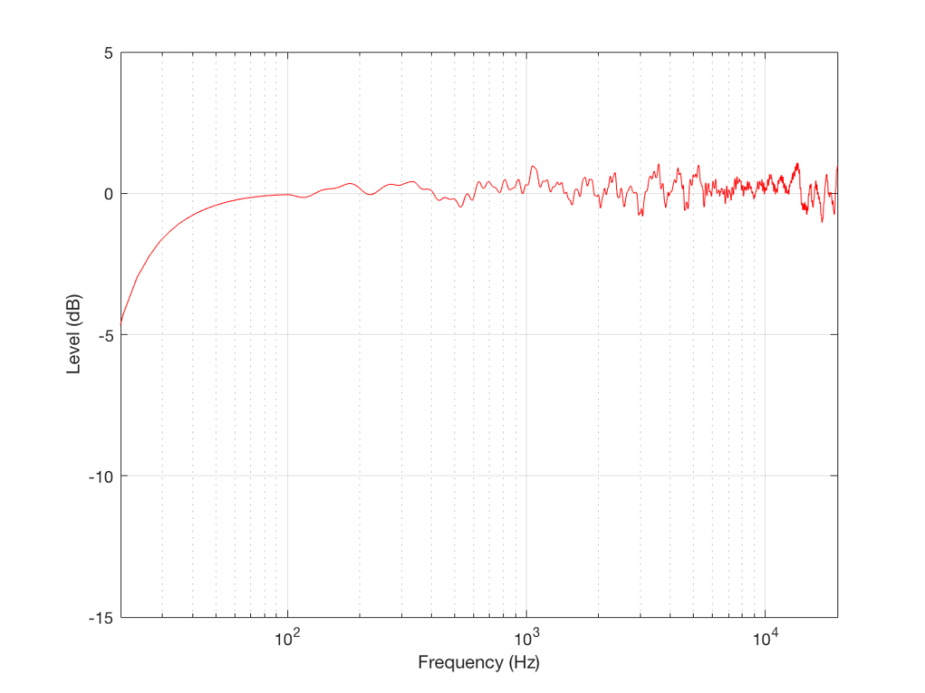
Figure 2: The on-axis, free-field magnitude response of a loudspeaker.
For example, take a look at the magnitude response shown in Figure 2, which is a real measurement of a real loudspeaker. This measurement was performed using a swept-sine (a sinusoidal wave with a frequency that changes smoothly over time, typically from low to high) with a microphone on-axis to the loudspeaker at a distance of 3 m. The measurement was time-windowed to remove the room reflections, and therefore can be considered to be a “free field” (a sound field that is free of reflections) measurement. However, the roll-off in the low end is actually a combination of the actual response of the loudspeaker and the artefacts of using a shorter time window. (We would have needed to use a much bigger room to get less influence from the time windowing.)
So, this plot ONLY tells us how the loudspeaker behaves at one point in infinite space, when we’re ONLY asking “how does the level of the loudspeaker’s output vary with changes in frequency and we ONLY play sinusoidal signals at one level.” This is all useful information, but we need to know more – otherwise, we’ll jump to conclusions about whether this loudspeaker sounds “good” or not.
Just like looking at ONLY the temperature of a cup of coffee, this doesn’t give us enough of the story to know how the loudspeaker will “sound” (no matter what a magazine reviewer will try and tell you…).
In other words, if we use reductionism to understand the problem, you simplify the question so much that the problem you wind up understanding is not the same as the thing you’re trying to understand in the first place.
For example, if we measure that same loudspeaker at a different angle (by rotating the loudspeaker and leaving the microphone in place) we’ll see a magnitude response like the one shown in Figure 3.
Figure 3: The free-field magnitude response of the same loudspeaker, measured at 90º off-axis.
This magnitude response is the output of the same loudspeaker at 90º off-axis, which might be what’s heading towards your side-wall. If your side wall is perfectly reflective, then this is therefore the magnitude response of your first reflection, which might be a bad thing if you think that it’s important.
So, when you’re looking at any one measurement of anything, you don’t have enough information to know enough to make a general evaluation. However, unfortunately, many people will run with this information and make the evaluation anyway. It’s data, and data doesn’t lie, so this tells the truth, right?
Wrong. Because it’s only a portion of the total truth.
For example, you can say that “organic food is good for me” but I have an allergy to peanuts. So if I eat organic peanuts, I have about 20 minutes to get to a hospital. Much longer than that and I need a funeral home instead. “Organic” is true, but not enough information for me to know whether or not it’ll be an uneventful meal.
In Part 1 of this series, I talked about how a binaural audio signal can (hypothetically, with HRTFs that match your personal ones) be used to simulate the sound of a source (like a loudspeaker, for example) in space. However, to work, you have to make sure that the left and right ears get completely isolated signals (using earphones, for example).
In Part 2, I showed how, with enough processing power, a large amount of luck (using HRTFs that match your personal ones PLUS the promise that you’re in exactly the correct location), and a room that has no walls, floor or ceiling, you can get a pair of loudspeakers to behave like a pair of headphones using crosstalk cancellation.
There’s not much left to do to create a virtual loudspeaker. All we need to do is to:
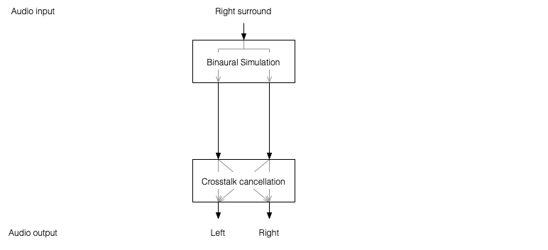
Take the signal that should be sent to a right surround loudspeaker (for example) and filter it using the HRTFs that correspond to a sound source in the location that this loudspeaker would be in. REMEMBER that this signal has to get to your two ears since you would have used your two ears to hear an actual loudspeaker in that location.
Send those two signals through a crosstalk cancellation processing system that causes your two loudspeakers to behave more like a pair of headphones.
Figure 1: A block diagram of the system described above.
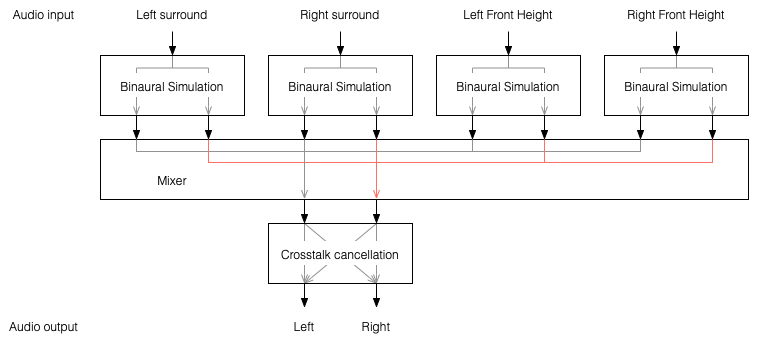
One nice thing about this system is that the crosstalk cancellation is only there to ensure that the actual loudspeakers behave more like headphones. So, if you want to create more virtual channels, you don’t need to duplicate the crosstalk cancellation processor. You only need to create the binaurally-processed versions of each input signal and mix those together before sending the total result to the crosstalk cancellation processor, as shown below.
Figure 2: You only need one crosstalk cancellation system for any number of virtual channels.
This is good because it saves on processing power.
So, there are some important things to realise after having read this series:
All “virtual” loudspeakers’ signals are actually produced by the left and right loudspeakers in the system. In the case of the Beosound Theatre, these are the Left and Right Front-firing outputs.
Any single virtual loudspeaker (for example, the Left Surround) requires BOTH output channels to produce sound.
If the delays (aka Speaker Distance) and gains (aka Speaker Levels) of the REAL outputs are incorrect at the listening position, then the crosstalk cancellation will not work and the virtual loudspeaker simulation system won’t work. How badly is doesn’t work depends on how wrong the delays and gains are.
The virtual loudspeaker effect will be experienced differently by different persons because it’s depending on how closely your actual personal HRTFs match those predicted in the processor. So, don’t get into fights with your friends on the sofa about where you hear the helicopter…
The listening room’s acoustical behaviour will also have an effect on the crosstalk cancellation. For example, strong early reflections will “infect” the signals at the listening position and may/will cause the cancellation to not work as well. So, the results will vary not only with changes in rooms but also speaker locations.
Finally, it’s worth nothing that, in the specific case of the Beosound Theatre, by setting the Speaker Distances and Speaker Levels for the Left and Right Front-firing outputs for your listening position, then you have automatically calibrated the virtual outputs. This is because the Speaker Distances and Speaker Levels are compensations for the ACTUAL outputs of the system, which are the ones producing the signal that simulate the virtual loudspeakers. This is the reason why the four virtual loudspeakers do not have individual Speaker Distances and Speaker Levels. If they did, they would have to be identical to the Left and Right Front-firing outputs’ values.
In Part 1, I talked at how a binaural recording is made, and I also mentioned that the spatial effects may or may not work well for you for a number of different reasons.
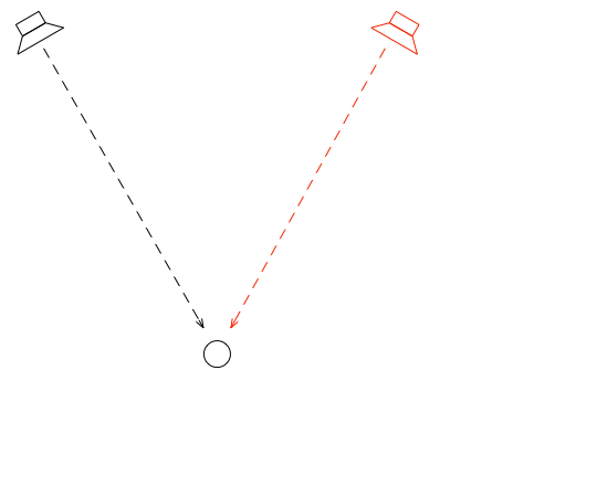
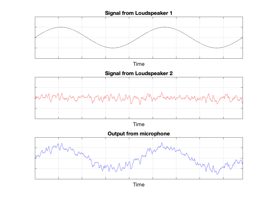
Let’s go back to the free field with a single “perfect” microphone to measure what’s happening, but this time, we’ll send sound out of two identical “perfect” loudspeakers. The distances from the loudspeakers to the microphone are identical. The only difference in this hypothetical world is that the two loudspeakers are in different positions (measuring as a rotational angle) as shown in Figure 1.
Figure 1: Two identical, “perfect” loudspeakers in a free field with a single “perfect” microphone.
In this example, because everything is perfect, and the space is a free field, then output of the microphone will be the sum of the outputs of the two loudspeakers. (In the same way that if your dog and your cat are both asking for dinner simultaneously, you’ll hear dog+cat and have to decide which is more annoying and therefore gets fed first…)
Figure 2: The output from the microphone is the sum of the outputs from the two loudspeakers. At any moment in time, the value of the top plot + the value of the middle plot = the value of the bottom plot.
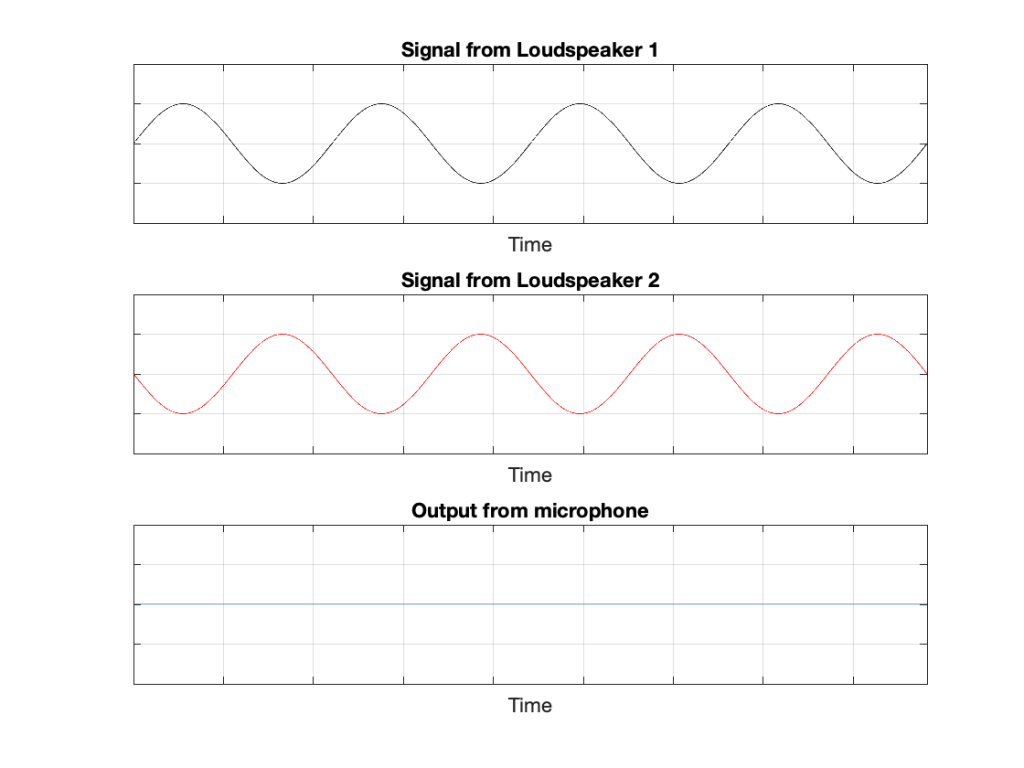
IF the system is perfect as I described above, then we can play some tricks that could be useful. For example, since the output of the microphone is the sum of the outputs of the two loudspeakers, what happens if the output of one loudspeaker is identical to the other loudspeaker, but reversed in polarity?
Figure 3: If the output of Loudspeaker 1 is exactly the same as the output of Loudspeaker 2 except for polarity, then the sum (the output of the microphone) is always 0.
In this example, we’re manipulating the signals so that, when they add together, you nothing at the output. This is because, at any moment in time, the value of Loudspeaker 2’s output is the value of Loudspeaker 1’s output * -1. So, in other words, we’re just subtracting the signal from itself at the microphone and we get something called “perfect cancellation” because the two signals cancel each other at all times.
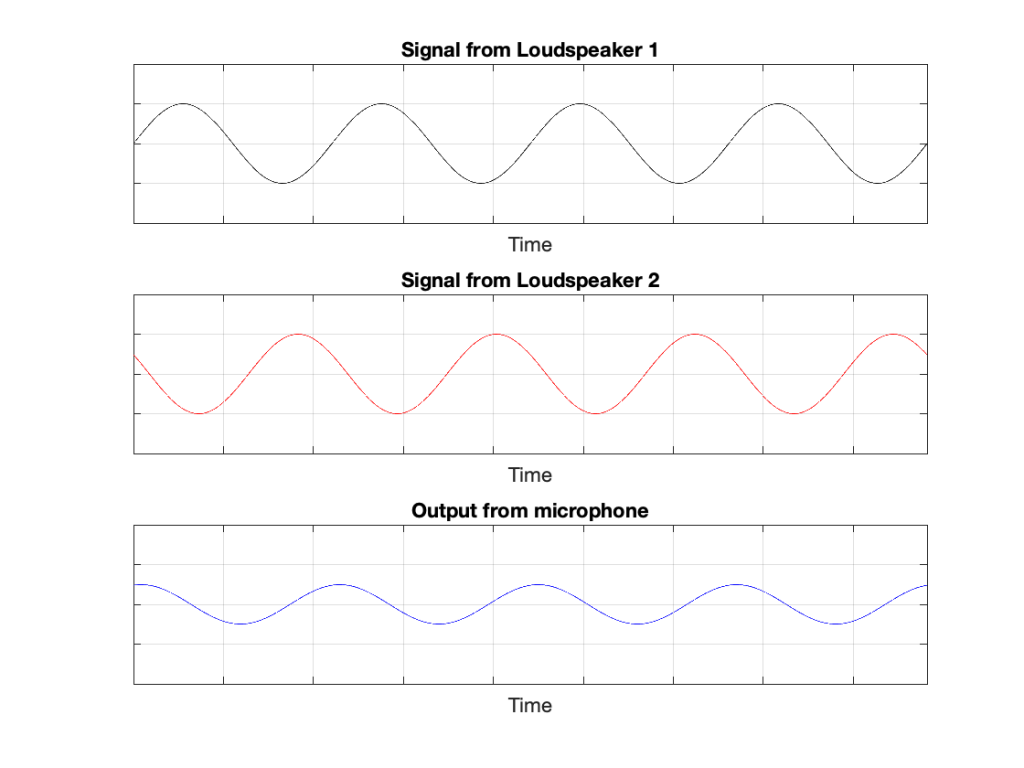
Of course, if anything changes, then this perfect cancellation won’t work. For example, if one of the loudspeakers moves a little farther away than the other, then the system is broken, as shown below.
Figure 4: A small shift in time in the output of Loudspeaker 2 cases the cancellation to stop working so well.
Again, everything that I’ve said above only works when everything is perfect, and the loudspeakers and the microphone are in a free field; so there are no reflections coming in and ruining everything.
We can now combine these two concepts:
using binaural signals to simulate a sound source in a location (although this would normally be done using playback over earphones to keep it simple) and
using signals from loudspeakers to cancel each other at some location in space as a
to create a system for making virtual loudspeakers.
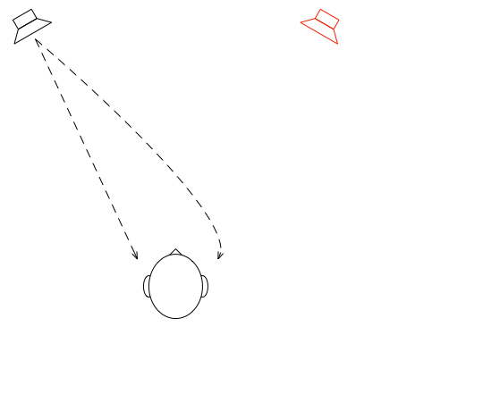
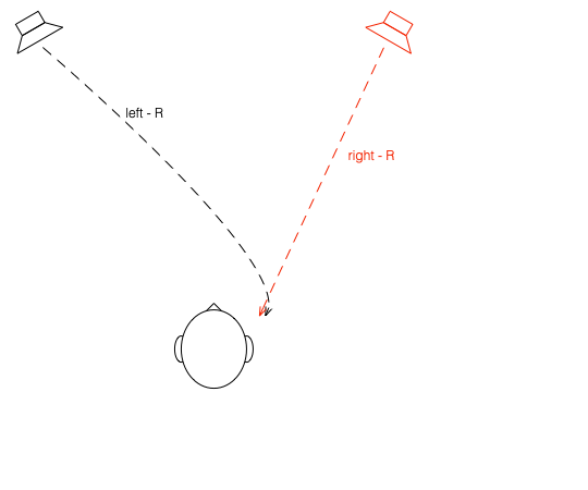
Let’s suspend our adherence to reality and continue with this hypothetical world where everything works as we want… We’ll replace the microphone with a person and consider what happens. To start, let’s just think about the output of the left loudspeaker.
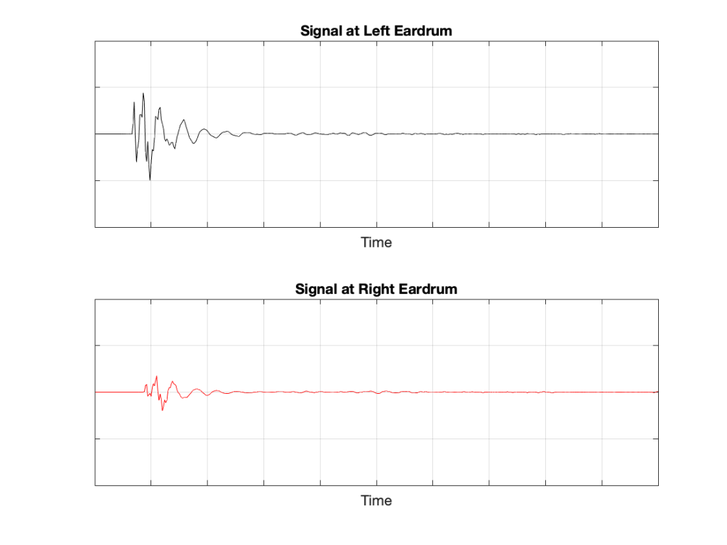
Figure 5: The output of the left loudspeaker reaches both ears with different time/frequency characteristics caused by the HRTF associated with that sound source location.
If we plot the impulse responses at the two ears (the “click” sound from the loudspeaker after it’s been modified by the HRTFs for that loudspeaker location), they’ll look like this:
Figure 6: The impulse responses of the HRTFs for a sound source at 30º left of centre.
What if were were able to send a signal out of the right loudspeaker so that it cancels the signal from the left loudspeaker at the location of the right eardrum?
Figure 7: What if we could cancel the signal from the left loudspeaker at the right ear using the right loudspeaker?
Unfortunately, this is not quite as easy as it sounds, since the HRTF of the right loudspeaker at the right ear is also in the picture, so we have to be a bit clever about this.
So, in order for this to work we:
Send a signal out of the left loudspeaker. We know that this will get to the right eardrum after it’s been messed up by the HRTF. This is what we want to cancel…
…so we take that same signal, and
filter it with the inverse of the HRTF of the right loudspeaker (to undo the effects of the HRTF of the right loudspeaker’s signal at the right ear)
filter that with the HRTF of the left loudspeaker at the right ear (to match the filtering that’s done by your head and pinna)
multiply by -1 (so that it will cancel when everything comes together at your right eardrum)
and send it out the right loudspeaker.
Hypothetically, that signal (from the right loudspeaker) will reach your right eardrum at the same time as the unprocessed signal from the left loudspeaker and the two will cancel each other, just like the simple example shown in Figure 3. This effect is called crosstalk cancellation, because we use the signal from one loudspeaker to cancel the sound from the other loudspeaker that crosses to the wrong side of your head.
This then means that we have started to build a system where the output of the left loudspeaker is heard ONLY in your left ear. Of course, it’s not perfect because that cancellation signal that I sent out of the right loudspeaker gets to the left ear a little later, so we have to cancel the cancellation signal using the left loudspeaker, and back and forth forever.
If, at the same time, we’re doing the same thing for the other channel, then we’ve built a system where you have the left loudspeaker’s signal in the left ear and the right loudspeaker’s signal in the right ear; just like a pair of headphones!
However, if you get any of these elements wrong, the system will start to under-perform. For example, if the HRTFs that I use to predict your HRTFs are incorrect, then it won’t work as well. Or, if things aren’t time-aligned correctly (because you moved) then the cancellation won’t work.
Devices such as the ‘stereoscope’ for representing photographs (and films) in three-dimensions have been around since the 1850s. These work by presenting two different photographs with slightly different perspectives two the two eyes. If the differences in the photographs are the same as the differences your eyes would have seen had you ‘been there’, then your brain interprets into a 3D image.
A similar trick can be done with sound sources. If two different sounds that exactly match the signals that you would have heard had you ‘been there’ are presented at your two ears (using a binaural recording) , then your brain will interpret the signals and give you the auditory impression of a sound source in some position in space. The easiest way to do this is to ensure that the signals arriving at your ears are completely independent using headphones.
The problem with attempting this with loudspeaker reproduction is that there is ‘crosstalk’ or ‘bleeding of the signals to the opposite ears’. For example, the sound from a correctly-positioned Left Front loudspeaker can be heard by your left ear and your right ear (slightly later, and with a different response). This interference destroys the spatial illusion that is encoded in the two audio channels of a binaural recording.
However, it might be possible to overcome this issue with some careful processing and assumptions. For example, if the exact locations of the left and right loudspeakers and your left and right ears are known by the system, then it’s (hypothetically) possible to produce a signal from the right loudspeaker that cancels the sound of the left loudspeaker in the right ear, and therefore you only hear the left channel in the left ear. (Of course, the cancelling signal of the right loudspeaker also bleeds to the left ear, so the left loudspeaker has to be used to cancel the cancellation signal of the right loudspeaker in the left ear, and so on…)
Using this ‘crosstalk cancellation’ processing, it becomes (hypothetically) possible to make a pair of loudspeakers behave more like a pair of headphones, with only the left channel in the left ear and the right in the right. Therefore, if this system is combined with the binaural recording / reproduction system, then it becomes (hypothetically) possible to give a listener the impression of a sound source placed at any location in space, regardless of the actual location of the loudspeakers.
Theory vs. Reality
It’s been said that the difference between theory and practice is that, in theory, there is no difference between theory and practice, whereas in practice, there is. This is certainly true both of binaural recordings (or processing) and crosstalk cancellation.
In the case of binaural processing, in order to produce a convincing simulation of a sound source in a position around the listener, the simulation of the acoustical characteristics of a particular listener’s head, torso, and (most importantly) pinnae (a.k.a. ‘ears’) must be both accurate and precise. (For the same reason that someone else should not try to wear my glasses.)
Similarly, a crosstalk cancellation system must also have accurate and precise ‘knowledge’ of the listener’s physical characteristics in order to cancel the signals correctly; but this information also crucially includes the exact locations of the
loudspeakers and the listener (we’ll conveniently pretend that the room you’re sitting in does not exist).
In the end, this means that a system with adequate processing power can use two loudspeakers to simulate a ‘virtual’ loudspeaker in another location. However, the details of that spatial effect will be slightly different from person to person (because we’re all shaped differently). Also, more importantly, the effect will only be experienced by a listener who is positioned correctly in front of the loudspeakers. Slight movements (especially from side-to-side, which destroys the symmetrical time-of-arrival matching of the two incoming signals) will cause the illusion to collapse.
Beosound Theatre gives you the option to choose Virtual Loudspeakers that appear to be located in four different positions: Left and Right Wide, and Left and Right Elevated. These signals are actually produced using the Left and Right front-firing outputs of the device using this combination of binaural processing and crosstalk cancellation in the Dolby Atmos processing system. If you are a single listener in the correct position (with the Speaker Distances and Speaker Levels adjusted correctly) then the Virtual outputs come very close to producing the illusion of correctly-located Surround and Front Height loudspeakers.
However, in cases where there is more than one listener, or where a single listener may be incorrectly located, it may be preferable to use the ‘side-firing’ and ‘up-firing’ outputs instead.
Beosound Theatre has a total of 11 possible outputs, seven of which are “real” or “internal” outputs and four of which are “virtual” loudspeakers. As with all current Beovision televisions, any input channel can be directed to any output by setting the Speaker Roles in the menus.
Internal outputs
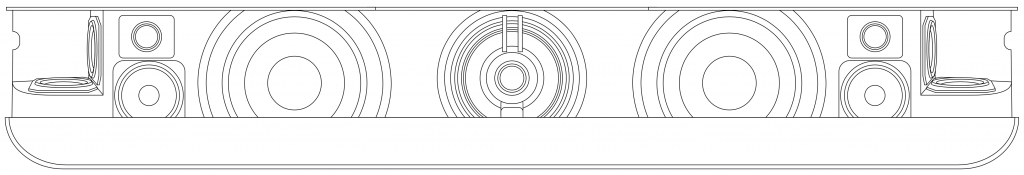
On first glance of the line drawing above it is easy to jump to the conclusion that the seven real outputs are easy to find, however this would be incorrect. The Beosound Theatre has 12 loudspeaker drivers that are all used in some combination of level and phase at different frequencies to all contribute to the total result of each of the seven output channels.
So, for example, if you are playing a sound from the Left front-firing output, you will find that you do not only get sound from the left tweeter, midrange, and woofer drivers as you might in a normal soundbar. There will also be some contribution from other drivers at different frequencies to help control the spatial behaviour of the output signal. This Beam Width control is similar to the system that was first introduced by Bang & Olufsen in the Beolab 90. However, unlike the Beolab 90, the Width of the various beams cannot be changed in the Beosound Theatre.
The seven internal loudspeaker outputs are
Front-firing: Left, Centre, and Right
Side-firing: Left and Right
Up-firing: Left and Right
Looking online, you may find graphic explanations of side-firing and up-firing drivers in other loudspeakers. Often, these are shown as directing sound towards a reflecting wall or ceiling, with the implication that the listener therefore hears the sound in the location of the reflection instead. Although this is a convenient explanation, it does not necessarily match real-life experience due to the specific configuration of your system and the acoustical properties of the listening room.
The truth is both better and worse than this reductionist view. The bad news is that the illusion of a sound coming from a reflective wall instead of the loudspeaker can occur, but only in specific, optimised circumstances. The good news is that a reflecting surface is not strictly necessary; therefore (for example) side-firing drivers can enhance the perceived width of the loudspeaker, even without reflecting walls nearby.
However, it can be generally said that the overall benefit of side- and up-firing loudspeaker drivers is an enhanced impression of the overall width and height of the sound stage, even for listeners that are not seated in the so-called “sweet spot” (see Footnote 1) when there is appropriate content mixed for those output channels.
Virtual outputs
Devices such as the “stereoscope” for representing photographs (and films) in three-dimensions have been around since the 1850s. These work by presenting two different photographs with slightly different perspectives two the two eyes. If the differences in the photographs are the same as the differences your eyes would have seen had you “been there”, then your brain interprets into a 3D image.
A similar trick can be done with sound sources. If two different sounds that exactly match the signals that you would have heard had you “been there” are presented at your two ears (using a binaural recording) , then your brain will interpret the signals and give you the auditory impression of a sound source in some position in space. The easiest way to do this is to ensure that the signals arriving at your ears are completely independent using headphones.
The problem with attempting this with loudspeaker reproduction is that there is “crosstalk” or “bleeding of the signals to the opposite ears”. For example, the sound from a correctly-positioned Left Front loudspeaker can be heard by your left ear and your right ear (slightly later, and with a different response). This interference destroys the spatial illusion that is encoded in the two audio channels of a binaural recording.
However, it might be possible to overcome this issue with some careful processing and assumptions. For example, if the exact locations of the left and right loudspeakers and your left and right ears are known by the system, then it’s (hypothetically) possible to produce a signal from the right loudspeaker that cancels the sound of the left loudspeaker in the right ear, and therefore you only hear the left channel in the left ear. (see Footnote 2)
Using this “crosstalk cancellation” processing, it becomes (hypothetically) possible to make a pair of loudspeakers behave more like a pair of headphones, with only the left channel in the left ear and the right in the right. Therefore, if this system is combined with the binaural recording / reproduction system, then it becomes (hypothetically) possible to give a listener the impression of a sound source placed at any location in space, regardless of the actual location of the loudspeakers.
Theory vs. Reality
It’s been said that the difference between theory and practice is that, in theory, there is no difference between theory and practice, whereas in practice, there is. This is certainly true both of binaural recordings (or processing) and crosstalk cancellation.
In the case of binaural processing, in order to produce a convincing simulation of a sound source in a position around the listener, the simulation of the acoustical characteristics of a particular listener’s head, torso, and (most importantly) pinnæ (a.k.a. “ears”) must be both accurate and precise. (see Footnote 3)
Similarly, a crosstalk cancellation system must also have accurate and precise “knowledge” of the listener’s physical characteristics in order to cancel the signals correctly; but this information also crucially includes the exact locations of the loudspeakers and the listener (we’ll conveniently pretend that the room you’re sitting in does not exist).
In the end, this means that a system with adequate processing power can use two loudspeakers to simulate a “virtual” loudspeaker in another location. However, the details of that spatial effect will be slightly different from person to person (because we’re all shaped differently). Also, more importantly, the effect will only be experienced by a listener who is positioned correctly in front of the loudspeakers. Slight movements (especially from side-to-side, which destroys the symmetrical time-of-arrival matching of the two incoming signals) will cause the illusion to collapse.
Beosound Theatre gives you the option to choose Virtual Loudspeakers that appear to be located in four different positions: Left and Right Wide, and Left and Right Elevated. These signals are actually produced using the Left and Right front-firing outputs of the device using this combination of binaural processing and crosstalk cancellation in the Dolby Atmos processing system. If you are a single listener in the correct position (with the Speaker Distances and Speaker Levels adjusted correctly) then the Virtual outputs come very close to producing the illusion of correctly-located Surround and Front Height loudspeakers.
However, in cases where there is more than one listener, or where a single listener may be incorrectly located, it may be preferable to use the “side-firing” and “up-firing” outputs instead.
Wrapping up
As I mentioned at the start, Beosound Theatre on its own has 11 outputs:
Front-firing: Left, Centre, and Right
Side-firing: Left and Right
Up-firing: Left and Right
Virtual Wide: Left and Right
Virtual Elevated: Left and Right
In addition to these, there are 8 wired Power Link outputs and 8 Wireless Power Link outputs for connection to external loudspeakers, resulting in a total of 27 possible output paths. And, as is the case with all Beovision televisions since Beoplay V1, any input channel (or output channel from the True Image processor) can be directed to any output, giving you an enormous range of flexibility in configuring your system to your use cases and preferences.
1. In the case of many audio playback systems, the “sweet spot” is directly in front of the loudspeaker pair or at the centre of the surround configuration. In the case of a Bang & Olufsen system, the “sweet spot” is defined by the user with the help of the Speaker Distance and Speaker Level adjustments.
2. Of course, the cancelling signal of the right loudspeaker also bleeds to the left ear, so the left loudspeaker has to be used to cancel the cancellation signal of the right loudspeaker in the left ear, and so on…
3. For the same reason that someone else should not try to wear my glasses.
If you you get an audiometry test done, you’ll be shown into a small room, about the size of a public bathroom stall. Someone will put a pair of headphones on you, and pass you a small handle with a button. Your instructions are to press the button if you hear a tone. Then the audiometrist will leave the room, closing the door, and you’ll suddenly realise that if there’s any noise in this room, it’s because you’re making it.
Then you hear a beep in your left ear. You press the button. You hear a quieter beep. Press. Quieter beep. Press…. …. …. Beep, press… …. …. …. Beep, press…. New frequency beep, loud again. Press… and so on.
What’s happening here is that you’re presented with a sine tone at some frequency, probably loud enough for you to hear. You press. The tone gets quieter, and you press again. Eventually, the tone is so quiet that you cannot hear it (this is normal) so you don’t press. So, the tone gets louder, and you press. Then it gets quieter again, until you can’t hear it again.
By crossing over that threshold of “can hear” and “can’t hear” a couple of times, the audiometrist finds out whether or not you got lucky… If you bottom out at the same level a couple of times in a row, then that’s your threshold of hearing at that frequency in that ear.
The frequency changes (usually by 1 octave, but sometimes less), and the whole process is repeated.
If you get a full test done, then this is probably done at 9 frequencies (250, 500, 1k, 1.5k, 2k, 3k, 4k, 6k, and 8kHz) in both ears individually – 18 tests in all.
You’ll then be given a sheet of paper, or at least shown a plot of your hearing threshold. Typically, if you have “normal” hearing (whatever that means) your thresholds will all be sitting on a horizontal line marked 0 dB. If you’re “better than normal” then you get a negative score, if you’re “worse than normal” you get a positive score.
What does this mean?
Let’s start over.
If a lot of people do this test, and we only test at 1 kHz, we’ll find out that, after the results are averaged, the group can hear the 1 kHz sine tone when the change in air pressure at the ear entrance is 20 µPa. We’re not going to talk about what this means other than to say that “sound is a change in air pressure over time, and that pressure is measured in pascals, abbreviated Pa”. Needless to say, 20 µPa is pretty quiet, since it’s the quietest sound a group of people can hear at 1 kHz when you take their average.
If you did that test at a much lower frequency, you would find out that people aren’t as good at hearing quiet sounds. In other words, at 100 Hz, the sine tone has to be louder than 20 µPa for people to hear it.
The same is true if you repeated the test at a much higher frequency – say, 10,000 Hz.
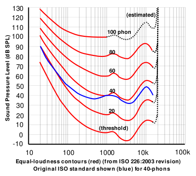
If you did this test at a lot of frequencies, then you’d find out that, on average, the threshold of hearing for a human follows the bottom red line of the plot in Figure 1, borrowed from Wikipedia.
Figure 1: The bottom red curve is the average threshold of hearing for a human being.
That bottom plot shows the threshold of hearing for different frequencies, plotted in dB SPL. Notice that, at 1 kHz, the line is at 0 dB SPL. This is because 0 dB SPL is defined to be the average threshold of hearing of a human at 1 kHz, which is 20 µPa. So, it’s not an accident…
Looking at that plot, you can see that, in order to hear a sine tone at 20 Hz, the tone has got to be more than 70 dB louder (that’s a LOT louder). So, a microphone “sees” a 73 dB SPL, 20 Hz sine tone as being louder than a 0 dB SPL, 1 kHz sine tone – but as far as you’re concerned, they’re both “the quietest sound you can hear” – therefore, they’re the same level.
If we take that threshold of hearing curve, and we play tones at those levels for those frequencies, then you should “just be able to” hear them. So, we’ll call those levels “0 dB” – since it’s the same as what is expected of you.
In other words, the piece of paper you got from the audiometrist tells you how much above or below that red threshold of hearing YOU sit.
Now, let’s back up a bit.
I said that, in your test, you only went up to 8 kHz. This is because, above that (and possibly even before that) the headphones might not be trust-worthy, and even a tiny movement (say a couple of millimetres) in the position of the headphones will have a (relatively) big effect on the level at your eardrum. So, rather than get people worried about losing their hearing at 20,000 Hz (when, in fact, they were actually just wearing the headphones 1 mm too far forward), you won’t get tested.
Notice how variable that threshold of hearing line is. There are big changes in level over the “audible” frequency range.
Remember that the threshold of hearing curve is an AVERAGE of a lot of people. Just like no one has 2.6 children, no one has this exact response. And, if you are some freak of nature and you DO have exactly that response, you don’t for long… we all get old…
Notice how that threshold of hearing curve only goes up to about 16 kHz, and above that it says “estimated”. See point #1.
Now, you should know that your ability to hear a sine tone at some frequency is defined as how your ability compares to an expectation based on an average, within a relatively small frequency band: 250 to 8 kHz.
Then you look at a textbook or you read a website that says “humans can hear from 20 Hz to 20 kHz”, which is not enough information to be either true or false… It’s like saying “humans are usually between 0 and 10 m tall” which is also sort of true, but also adequately vague to be potentially worse-than-useless information.
The truth is, unfortunately, much more complicated… However, it’s fair to say that, in order for you to just hear a sine tone at 20 kHz, it would have to be much, much louder than one at 1 kHz. In fact, if I played a 20 kHz sine tone loud enough for you to hear, measured that level, and then played a 1 kHz sine tone for you at the same level, you’d probably punch me – after you had passed out due to the pain, woken up, hunted me down, and found me… (I’d already have run away by then….)
So what?
We humans like nice, tidy, answers. “It will rain tomorrow” is preferable to “there is a 70 – 80% chance of scattered showers in the afternoon tomorrow”. We even get mad when the information is correct, but we interpret it tidily… For example, we’ll complain about getting rained on in the middle of our hike, when there was only a 10% chance of rain. On the other hand, if there was a 10% chance of winning 1 Million dollars in the lottery, we’d all buy a ticket.
Anyways, once-upon-a-time, when the committee for inventing the compact disc was holding meetings, they said “what should the sampling rate be?” and someone said “at least 40 kHz, because we can hear up to 20 kHz”. (The reason it’s 44100 is related to the fact that the bits were stored as black and white stripes on video tape, and NTSC and PAL come close to meeting each other close to that number, when you look at the numbers of lines per field and frames per second.)
Of course, like any first-generation thing, digital recording equipment wasn’t very good at the start (back around 1980 or so) – so the first DDD recordings that were released on CD sounded… well…. weird. There was quantisation distortion because they hadn’t figured out dither yet, only 12 or 13 of the bit values were working properly on the ADC’s, the anti-aliasing filters were implemented as analogue circuits, so they let some stuff through that aliased, and they rang (“sang along”) with the signal at a high frequency… All of that added up to “weird” – possibly even “bad”. Then, people who had good equipment (high-end turntables or, even better, 1/4″ tape running at 30 ips) listened to this new format, decided it was bad, and that was that.
Some of them asked “why is is bad?” and one answer they came up with was the band limiting… If the system can’t capture or store or play materials above 20 kHz, then it’s useless… Right? Maybe…
Then, instruments were put in front of measurement microphones and spectra were measured – and the proof was in. Trumpets with harmon (wah-wah) mutes, when pointing directly at the microphone, contain harmonics as high as 50 kHz! This must explain why CDs sound bad! Right? Maybe…
Then Rupert Neve did a demo at an AES (Audio Engineering Society) convention where he played people two tones. Both were at 7 kHz, but one was a sine wave and the other was a square wave (at some level). The question was: have a listen and tell me which is which. The results were the same as if everyone was just guessing. (Remember that, in order to make a square wave, you need to add odd harmonics – so the lowest-frequency content difference between a 7 kHz sine wave and a 7 kHz square wave is at 21 kHz.) Proof that we don’t need to go above 20 kHz, right? Maybe…
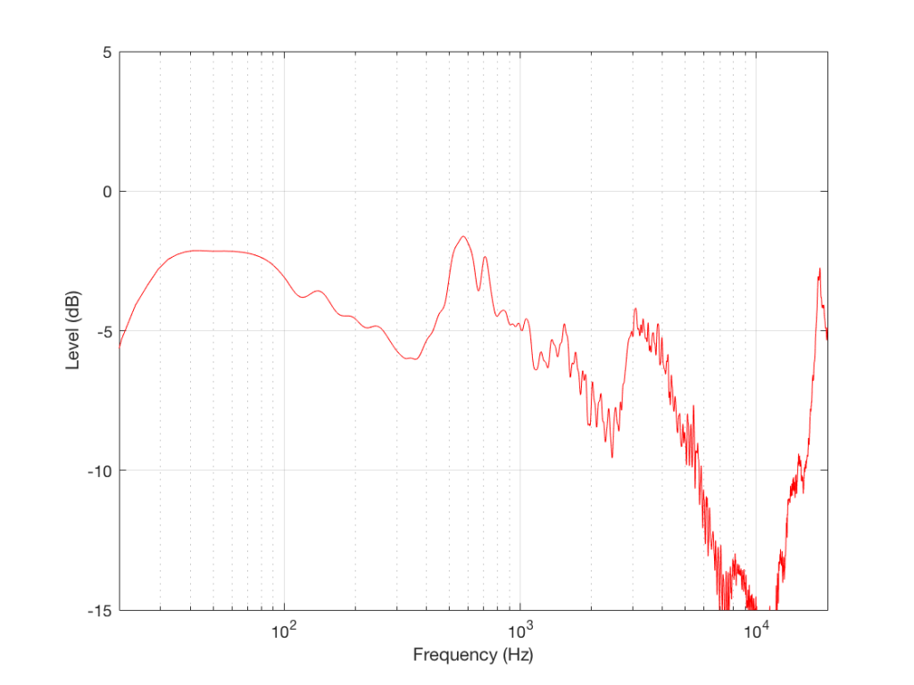
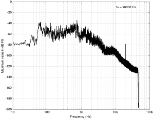
Some years ago, I took some “high resolution” audio files and measured their spectral content. One particularly interesting result is shown in Figures 2, below.
Figure 2: The spectral content of a 96/24 “high resolution” audio file I bought.
Look at that spike in the top end – around 20 kHz. What musical instrument makes that sound? The answer is “no musical instrument makes that sound – at least none of the baroque instruments in that recording make that sound. As I wrote back in 2014:
If you’re wondering what it might be, I asked a bunch of smart friends, and the best explanation we can come up with is that it’s noise from a switched-mode power supply that is somehow bleeding into the recording. HOW it’s bleeding into the recording is a potentially interesting question for recording engineers. One possibility is that one of the musicians was charging up a phone in the room where the microphones were – and the mic’s just picked up the noise. Another possibility is that the power supply noise is bleeding electrically into the recording chain – maybe it’s a computer power supply or the sound card and the manufacturer hasn’t thought about isolating this high frequency noise from the audio path. Or, maybe it’s something else.
Interestingly, this is a conflict of two engineers. The designer of the power supply (assuming that’s what it is…) said “I’ll put the switching frequency above 20 kHz so that no one will hear it” and the recording engineer said “I’ll record this at 96 kHz so that people can get the content they’re missing…” The problem is that the content you’re missing is something you don’t want…
Similarly, if you listen to Eric Clapton’s “Unplugged” album with headphones or loudspeakers that have a low-enough low-frequency range, you’ll hear a loud thump, thump, thump going along with the music. This is the sound of someone tapping their foot on a temporary stage floor, shaking a vocal microphone. In my not-very-humble opinion, that should never have made it out to the public release. However, my guess is that the speakers it was mastered on didn’t go low enough… (OR, it was an artistic decision, and I would have done it differently.) Assuming that I’m right, then this is a second example where a “better” system sounds “worse”.
Of course, through all of this, I have assumed that your loudspeakers or headphones can produce the signals that we’re talking about in the direction that you’re sitting in, and that those signals are not being masked by other sounds in the room (like phone chargers singing…) However, to complicate things with reality would just be too far to go today…
Conclusions?
I don’t have any, but I have some questions and (as usual) some opinions…
Does a harmon mute on a trumpet produce energy at 50 kHz, if you’re sitting right in front of it? Yes.
Do you want to sit right in front of a trumpet with a harmon mute? Debatable.
Can a high-res audio recording include the sound of a phone charger? Yes.
Do you want to have an expensive recording of a baroque ensemble with obligato phone charger? Probably not – the charger is not in Buxtehude’s original score as far as I can see.
Can you hear the difference between a 7 kHz sine and a 7 kHz square wave? Depends on the speaker / headphone, the listening position, the background noise level, and whether or not you were out clubbing last night. Heads or tails?
Will you feel better by knowing that your file contains “audio” content above 20 kHz? Probably. Placebos have been known to work bigger miracles than this. (But don’t forget the stuff I said about sampling rate converters earlier…)