This episode of The Infinite Monkey Cage is worth a listen if you’re interested in the history of recording technologies.
There’s one comment in there by Brian Eno that I COMPLETELY agree with. He mentions that we invented a new word for moving pictures: “movies” to distinguish them from the live equivalent, “plays”. But we never really did this for music… Unless, of course, you distinguish listening to a “concert” from listening to a “recording” – but most of us just say “I’m listening to music”.
It is often the case that you have to convert a floating point representation to a fixed point representation. For example, you’re doing some signal processing like changing the volume or adding equalisation, and you want to output the signal to a DAC or a digital output.
The easiest way to do this is to just send the floating point signal into the DAC or the S/PDIF transmitter and let it look after things. However, in my experience, you can’t always trust this. (I’ll explain why in a later posting in this series.) So, if you’re a geek like me, then you do this conversion yourself in advance to ensure you’re getting what you think you’re getting.
To start, we’ll assume that, in the floating point world, you have ensured that your signal is scaled in level to have a maximum amplitude of ± 1.0. In floating point, it’s possible to go much higher than this, and there’re no serious reason to worry going much lower (see this posting). However, we work with the assumption that we’re around that level.
So, if you have a 0 dB FS sine wave in floating point, then its maximum and minimum will hit ±1.0.
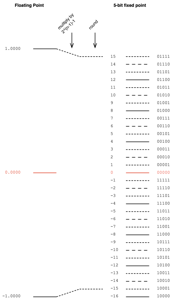
Then, we have to convert that signal with a range of ±1.0 to a fixed point system that, as we already know, is asymmetrical. This means that we have to be a little careful about how we scale the signal to avoid clipping on the positive side. We do this by multiplying the ±1.0 signal by 2^(nBits-1)-1 if the signal is not dithered. (Pay heed to that “-1” at the end of the multiplier.)
Let’s do an example of this, using a 5-bit output to keep things on a human scale. We take the floating point values and multiply each of them by 2^(5-1)-1 (or 15). We then round the signals to the nearest integer value and save this as a two’s complement binary value. This is shown below in Figure 1.
Figure 1. Converting floating point to a 5-bit fixed point value without dither.
As should be obvious from Figure 1, we will never hit the bottom-most fixed point quantisation level (unless the signal is asymmetrical and actually goes a little below -1.0).
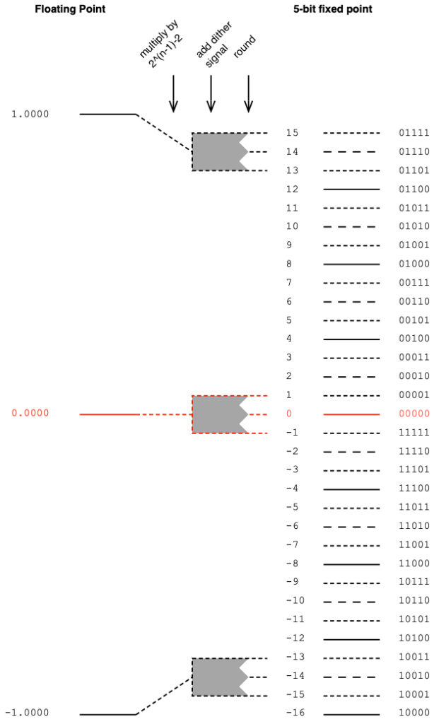
If you choose to dither your audio signal, then you’re adding a white noise signal with an amplitude of ±1 quantisation level after the floating point signal is scaled and before it’s rounded. This means that you need one extra quantisation level of headroom to avoid clipping as a result of having added the dither. Therefore, you have to multiply the floating point value by 2^(nBits-1)-2 instead (notice the “-2” at the end there…) This is shown below in Figure 2.
Figure 2. Converting floating point to a 5-bit fixed point value with dither.
Of course, you can choose to not dither the signal. Dither was a really useful thing back in the days when we only had 16 reliable bits to work with. However, now that 24-bit signals are normal, dither is not really a concern.
In Part 1, I talked about different options for converting a quantised LPCM audio signal, encoded with some number of bits into an encoding with more bits. In this posting, we’ll look at a trick that can be used when you combine these options.
To start, made two signals:
“Signal 1” is a sinusoidal tone with a frequency of 100 Hz. It has an amplitude of ±1, but then encoded it as a quantised 8-bit signal, so in Figure 1, it looks like it has an amplitude of ±127 (which is 2^(nBits-1)-1)
“Signal 2” is a sinusoidal tone with a frequency of 1 kHz and the same amplitude as Signal 1.
Both of these two signals are plotted on the left side of Figure 1, below. On the right, you can see the frequency content of the two signals as well. Notice that there is plenty of “garbage” at the bottom of those two plots. This is because I just quantised the signals without dither, so what you’re seeing there is the frequency-domain artefacts of quantisation error.
Figure 1. Two sinusoidal waveforms with different frequencies. Both are 8-bit quantised without dither.
If I look at the actual sample values of “Signal 1” for the first 10 samples, they look like the table below. I’ve listed them in both decimal values and their binary representations. The reason for this will be obvious later.
Sample number
Sample value (decimal)
Sample Value (binary)
1
0
00000000
2
2
00000010
3
3
00000011
4
5
00000101
5
7
00000111
6
8
00001000
7
10
00001010
8
12
00001100
9
13
00001101
10
15
00001111
Let’s also look at the first 10 sample values for “Signal 2”
Sample number
Sample value (decimal)
Sample Value (binary)
1
0
00000000
2
17
00010001
3
33
00100001
4
49
00110001
5
63
00111111
6
77
01001101
7
90
01011010
8
101
01100101
9
110
01101110
10
117
01110101
The signals I plotted above have a sampling rate of 48 kHz, so there are a LOT more samples after the 10th one… however, for the purposes of this posting, the ten values listed in the tables above are plenty.
At the end of the Part 1, I talked about the Most and the Least Significant Bits (MSBs and LSBs) in a binary number. In the context of that posting, we were talking about whether the bit values in the original signal became the MSBs (for Option 1) or the LSBs (for Option 3) in the new representation.
In this posting, we’re doing something different.
Both of the signals above are encoded as 8-bit signals. What happens if we combine them by just slamming their two values together to make 16-bit numbers?
For example, if we look at sample #10 from both of the tables above:
Signal 1, Sample #10 = 00001111
Signal 2, Sample #10 = 01110101
If I put those two binary numbers together, making Signal 1 the 8 MSBs and Signal 2 the 8 LSBs then I get
0000111101110101
Note that I formatted them with bold and italics just to make it easier to see them. I could have just written 0000111101110101 and let you figure it out.
Just to keep things adequately geeky, you should know that “slamming their values together” is not the correct term for what I’ve done here. It’s called binary concatenation.
Another way to think about what I’ve done is to say that I converted Signal 1 from an 8-bit to a 16-bit number by zero-padding, and then I added Signal 2 to the result.
Yet another way to think of it is to say that I added about 48 dB of gain to Signal 1 (20*log10(2^8) = about 48.164799306236993 dB of gain to be more precise…) and then added Signal 2 to the result. (NB. This is not really correct, as is explained below.)
However, when you’re working with the numbers inside the computer’s code, it’s easier to just concatenate the two binary numbers to get the same result.
If you do this, what do you get? The result is shown in Figure 2, below.
Figure 2. The binary concatenated result of Signal 1 and Signal 2
As you can see there, the numbers on the y-axis are MUCH bigger. This is because of the bit-shifting done to Signal 1. The MSBs of a 16-bit number are 256 times bigger in decimal world than those of an 8-bit number (because 2^8 = 256).
In other words, the maximum value in either Signal 1 or Signal 2 is 127 (or 2^(8-1)-1) whereas the maximum value in the combined signal is 32767 (or 2^(16-1)-1).
The table below shows the resulting first 10 values of the combined signal.
Sample number
Sample value (decimal)
Sample Value (binary)
1
0
0000000000000000
2
529
0000001000010001
3
801
0000001100100001
4
1329
0000010100110001
5
1855
0000011100111111
6
2125
0000100001001101
7
2650
0000101001011010
8
3173
0000110001100101
9
3438
0000110101101110
10
3957
0000111101110101
Why is this useful? Well, up to now, it’s not. But, we have one trick left up our sleeve… We can split them apart again, taking that column of numbers on the right side of the table above, cut each one into two 8-bit values, and ta-da! We get out the two signals that we started with!
Just to make sure that I’m not lying, I actually did all of that and plotted the output in Figure 3. If you look carefully at the quantisation error artefacts in the frequency-domain plots, you’ll see that they’re identical to those in Figure 1. (Although, if they weren’t, then this would mean that I made a mistake in my Matlab code…)
Figure 3. The two signals after they’ve been separated once again.
So what?
Okay, this might seem like a dumb trick. But it’s not. This is a really useful trick in some specific cases: transmitting audio signals is one of the first ones to come to mind.
Let’s say, for example, that you wanted to send audio over an S/PDIF digital audio connection. The S/PDIF protocol is designed to transmit two channels of audio with up to 24-bit LPCM resolution. Yes, you can do different things by sending non-LPCM data (like DSD over PCM (DoP) or Dolby Digital-encoded signals, for example) but we won’t talk about those.
If you use this binary concatenation and splitting technique, you could, for example, send two completely different audio signals in each of the audio channels on the S/PDIF. For example, you could send one 16-bit signal (as the 16 MSBs) and a different 8-bit signal (as the LSBs), resulting in a total of 24 bits.
On the receiving end, you split the 24-bit values into the 16-bit and 8-bit constituents, and you get back what you put in.
(Or, if you wanted to get really funky, you could put the two 8-bit leftovers together to make a 16-bit signal, thus transmitting three lossless LPCM 16-bit channels over a stream designed for two 24-bit signals.)
However, if you DON’T split them, and you just play the 24-bit signal into a system, then that 8-bit signal is so low in level that it’s probably inaudible (since it’s at least 93 dB below the peak of the “main” signal). So, no noticeable harm done!
Hopefully, now you can see that there are lots of potential uses for this. For example, it could be a sneaky way for a record label to put watermarking into an audio signal, for example. Or you could use it to send secret messages across enemy lines, buried under a recording of the Alvin and the Chipmunk’s cover of “Achy Breaky Heart”. Or you could use it for squeezing more than two channels out of an S/PDIF cable for multichannel audio playback.
One small issue…
Just to be clear, I actually used Matlab and did all the stuff I said above to make those plots. I didn’t fake it. I promise!
But if you’re looking carefully, you might notice two things that I also noticed when I was writing this.
I said above that, by bit-shifting Signal 1 over by 8 bits in the combined signal, this makes it 48 dB louder than Signal 2. However, if you look at the frequency domain plot in Figure 2, you’ll notice that the 1 kHz tone is about 60 dB lower than the 100 Hz tone. You’ll also notice that there are distortion artefacts on the 1 kHz signal at 3 kHz, 5 kHz and so on – but they’re not there in the extracted signal in Figure 3. So, what’s going on?
To be honest, when I saw this, I had no idea, but I’m lucky enough to work with some smart people who figured it out.
If you go back to the figures in Part 1, you can see that the MSB of a sample value in binary representation is used as the “sign” of the value. In other words, if that first bit is 0, then it’s a positive value. If it’s a 1 then it’s a negative value. This is known as a “two’s complement” representation of the signal.
When we do the concatenation of the two sample values as I showed in the example above, the “sign” bit of the signal that becomes the LSBs of the combined signal no longer behaves as a +/- sign. So, the truth is that, although I said above that it’s like adding the two signals – it’s really not exactly the same.
If we take the signal combined through concatenation and subtract ONLY the bit-shifted version of Signal 1, the result looks like this:
Figure 4. The difference between the combined signals shown in Figure 3 and Signal 1, after it’s been bit-shifted (or zero-padded) by 8 LSBs.
Notice that the difference signal has a period of 1 ms, therefore its fundamental is 1 kHz, which makes sense because it’s a weirdly distorted version of Signal 2, which is a 1 kHz sine tone.
However, that fundamental frequency has a lower level than the original sine tone (notice that it shows up at about -60 dB instead of -48 dB in Figure 2). In addition, it has a DC offset (no negative values) and it’s got to have some serious THD to be that weird looking. Since it’s a symmetrical waveform, its distortion artefacts consist of only odd multiples of the fundamental.
Therefore, when I stated above that you’re “just” adding the two signals together, so there’s no harm done if you don’t separate them at the receiving end. This was a lie. But, if your signal with the MSBs has enough bits, then you’ll get away with it, since this pushes the second signal further down in level.
This is the first of a series of postings about strategies for converting from one bit depth to another, including conversion back and forth between fixed point and floating point encoding. It’ll be focusing on a purely practical perspective, with examples of why you need to worry about these things when you’re doing something like testing audio devices or transmission systems.
As we go through this, it might be necessary to do a little review, which means going back and reading some other postings I’ve done in the past if some of the concepts are new. I’ll link back to these as we need them, rather than hitting you with them all at once.
To start, if you’re not familiar with the concept of quantisation and bit depth in an LPCM audio signal, I suggest that you read this posting.
Now that you’re back, you know that if you’re just converting a continuous audio signal to a quantised LPCM version of it, the number of bits in the encoded sample values can be thought of as a measure of the system’s resolution. The more bits you have, the more quantisation steps, and therefore the better the signal to noise ratio.
However, this assumes that you’re using as many of the quantisation steps as possible – in other words, it assumes that you have aligned levels so that the highest point in the audio signal hits the highest possible quantisation step. If your audio signal is 6 dB lower than this, then you’re only using half of your available quantisation values. In other words, if you have a 16-bit ADC, and your audio signal has a maximum peak of -6 dB FS Peak, then you’ve done a 15-bit recording.
But let’s say that you already have an LPCM signal, and you want to convert it to a larger bit depth. A very normal real-world example of this is that you have a 16-bit signal that you’ve ripped from a CD, and you export it as a 24-bit wave file. Where do those 8 extra bits come from and where do they go?
Generally speaking, you have 3 options when you do this “conversion”, and the first option I’ll describe below is, by far the most common method.
Option 1: Zero padding
Let’s simplify the bit depths down to human-readable sizes. We’ll convert a 3-bit LPCM audio signal (therefore it has 2^3 = 8 quantisation steps) into a 5-bit representation (2^5 = 32 quantisation steps), instead of 16-bit to 24-bit. That way, I don’t have to type as many numbers into my drawings. The basic concepts are identical, I’ll just need fewer digits in this version.
The simplest method to do is to throw some extra zeros on the right side of our original values, and save them in the new format. A graphic version of this is shown in Figure 1.
Figure 1. Zero-padding to convert to a higher bit depth.
There are a number of reasons why this is a smart method to use (which also explains why this is the most common method).
The first is that there is no change in signal level. If you have a 0 dB FS Peak signal in the 3-bit world, then we assume that it hits the most-negative value of 100. If you zero-pad this, then the value becomes 10000, which is also the most-negative value in the 5-bit world. If you’re testing with symmetrical signals (like a sinusoidal tone) then you never hit the most-negative value, since this would mean that it would clip on the positive side. This might result in a test that’s worth talking about, since sinusoidal tone that hits 011 and is then converted to 01100. In the 5-bit world, you could make a tone that is a little higher in level (by 3 quantisation levels – those top three dotted lines on the right side of Figure 1), but that difference is very small in real life, so we ignore it. The biggest reason for ignoring this is that this extra “headroom” that you gain is actually fictitious – it’s an artefact of the fact that you typically test signal levels like this with sine tones, which are symmetrical.
The second reason is that this method gives you extra resolution to attenuate the signal. For example, if you wanted to make a volume knob that only attenuated the audio signal, then this conversion method is a good way to do it. (For example, you send a 16-bit digital signal into the input of a loudspeaker with a volume controller. You zero-pad the signal to 24-bit and you now have the ability to reduce the signal level by 141 dB instead of just 93 dB (assuming that you’re using dither…). This is good if the analogue dynamic range of the rest of the system “downstream” is more than 93 dB.) The extra resolution you get is equivalent to 6 dB * each extra bit. So, in the system above:
(5 bits – 3 bits) = 2 extra bits 2 extra bits * 6 dB = 12 dB extra resolution
There is one thing to remember when doing it this way, that you may consider to be a disadvantage. This is the fact that you can’t increase the gain without clipping. So, let’s say that you’re building a digital equaliser or a mixer in a fixed-point system, then you can’t just zero-pad the incoming signal and think that you can boost signals or add them. If you do this, you’ll clip. So, you would have to zero-pad at the input, then attenuate the signal to “buy” yourself enough headroom to increase it again with the EQ or by mixing.
Option 2
The second option is, in essence, the same as the trick I just explained in the previous paragraph. With this method, you don’t ONLY pad the right side of the values with zeros, you pad the values on the left as well with either a 1 or a 0, depending on whether the signals are positive or negative. This means that your “old” value is inserted into the middle of the new value, as shown below in Figure 2. (In this 3- to 5-bit example, this is identical to using option 1, and then dropping the signal level by 6 dB (1 of the 2 bits)).
If your conversion to the bigger bit depth is done inside a system where you know what you’ve done, and if you need room to scale the level of the signal up and down, this is a clever and simple way to do things. There are some systems that did this in the past, but since it’s a process that’s done internally, and we normal people sit outside the system, there’s no real way for us to know that they did it this way.
(For example, I once heard through the grapevine that there was a DAW that imported 24-bits into a 48-bit fixed point processing system, where they padded the incoming files with 12 bits on either side to give room to drop levels on the faders and also be able to mix a lot of full-scale signals without clipping the output.)
Option 3
I only add the third option as a point of completion. This is an unusual way to do a conversion, and I only personally know of one instance where it’s been used. This only means that it’s not a common way to do things – not that NO ONE does it.
In this method, all the padding is done on the left side of the binary values, as shown below in Figure 3.
If we’re thinking along the same lines as in Options 1 and 2, then you could say that this system does not add resolution to attenuate signals, but it does give you the option to make them louder.
However, as we’ll see in Part 2 of this series, there is another advantage to doing it this way…
Nota Bene
I’ve written everything above this line, intentionally avoiding a couple of common terms, but we’ll need those terms in our vocabulary before moving on to Part 2.
If you look at the figures above, and start at the red 0 line, as you go upwards, the increase in signal can be seen as an increase in the left-most bits in each quantisation value. Reading from left-to-right, the first bit tells us whether the value is positive (0) or negative (1), but after this (for the positive values) the more 1s you have on the left, the higher the level. This is why we call them the Most Significant Bits or MSBs. Of course, this means that the last bit on the right is the Least Significant Bit or LSB.
This means that I could have explained Option 1 above by saying:
The three bits of the original signal become the three MSBs of the new signal.
… which also tells us that the signal level will not drop when converted to the 5-bit system.
Or I could have explained Option 3 by saying:
The three bits of the original signal become the three LSBs of the new signal.
.. which also tells us that the signal level will drop when converted to the 5-bit system.
Being able to think in terms of LSBs and MSBs will be helpful later.
Finally… yes, we will talk about Floating Point representations. Later. But if you can’t wait, read this in the meantime.
I mentioned in this posting that lately I’ve been doing some measurements of a DUT that:
required a frequency analysis with a very big dynamic range
… which meant that I was testing it using a sine tone with a frequency that was exactly the same as an FFT bin’s frequency centre
… and the sine tone had to be sent through the device by playing a standard audio file (wav and/or FLAC)
So, I did this, but I saw some weirdness that I didn’t expect down in the noise floor of the FFT output. Whenever I’m testing something and I see something weird, I start working my way back through the audio chain to verify that the weirdness is coming from the thing that I’m testing, and not from my test system itself.
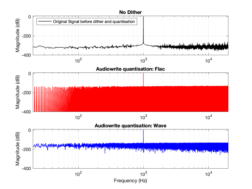
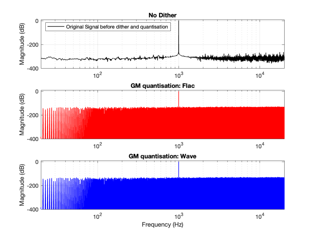
So, the first step was to do of an FFT of both the .wav and the .flac files that I was sending through the DUT. The results of this test looked something like Figure 1.
Figure 1.
Before I go further, let’s clarify exactly what I did to generate those three plots.
Using Matlab, I made a sine wave with a frequency identical to an FFT bin that was a close as possible to 997 Hz as I could get with a 65,536-point FFT at 48 kHz. (See this posting for more information about this.)
I exported the signal using Matlab’s “audiowrite” function, both as a 24-bit wav and a 24-bit FLAC.
I imported the two files back into Matlab
I ran an FFT on the original, and the two imported files
I would not expect the bottom two plots to be as “good” as the top plot, since they’ve been reduced to a 24-bit fixed point version of the original floating-point signal. However, there are two things to notice in Figure 1.
The most important thing is that the FLAC and WAVE imports produce different results. This is weird.
The less-important (but more interesting, later…) thing is that, for the FLAC import, every odd-numbered FFT bin is -∞ dB, which means that there is absolutely NO energy at those frequencies.
First things first
Let’s address that first issue first. The FFTs show us that the signals coming back from the .wav and .flac import are different. But I’m interested in (1) how they’re different and (2) why they’re different.
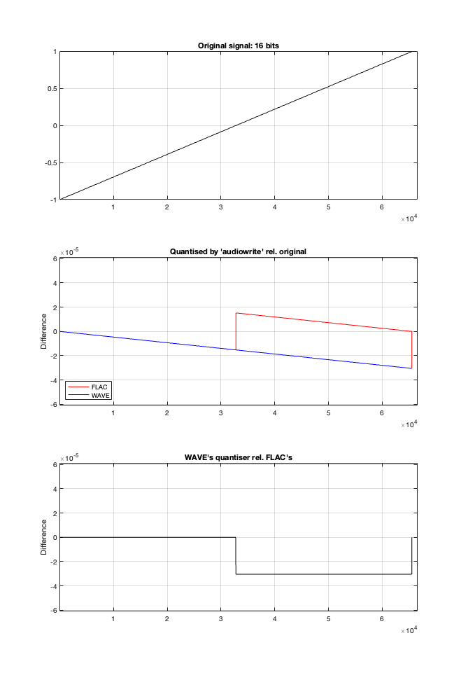
Let’s try to answer the first question first. I made a linear ramp that had the same number of samples as the number of quantisation values and had a range of -1 to 1 (just like my sine wave…). So, to test a 16-bit export, I made a ramp that was 216 = 65,536 samples long (shown in the top plot in Figure 2). To test a 24-bit export, the ramp was 224 samples long.
In theory, if I export this ramp to a file type with the matching number of bits, then each sample should quantise to the next quantisation level from the bottom to the top. I then exported this ramp out to .wav and .flac, imported it again, and looked at the result, which is shown in Figure 2.
Figure 2.
If I subtract the results of the imported files from the original, I get the result shown in the middle plot in Figure 2. I would NOT expect either the .wav or the .flac to be identical to the original, since information is lost in the export to a 16- or 24-bit fixed point LPCM format. However, I WOULD expect the .wav and .flac to be the same, which they obviously aren’t.
As can be seen in the bottom plot in Figure 2, there is a 1-quantisation level difference between the .wav and .flac files for signal values higher than 0.
Now the question is whether this difference is inherent in the file format, or if something else is going on. To test this, I did the same test on the 997-ish Hz sine wave (again) without dither, but with my own quantisation (using the code shown in this post). The result of this test is shown in Figure 3.
Figure 3.
As you can see there, the imported .wav and .flac files behave identically. But, if you look carefully and compare to the .flac version in Figure 1, you’ll see that they’re different from THAT version.
The fact that the red and blue plots in Figure 3 are identical tell me that .wav and .flac are identical.
The fact that my quantisation results in identical results in .wav and .flac, but are different from Matlab’s “audiowrite” results (which produces .wav and .flac files that are different from each other) tells me that Matlab’s quantisation is different for .wav and .flac – and different from what I’m doing.
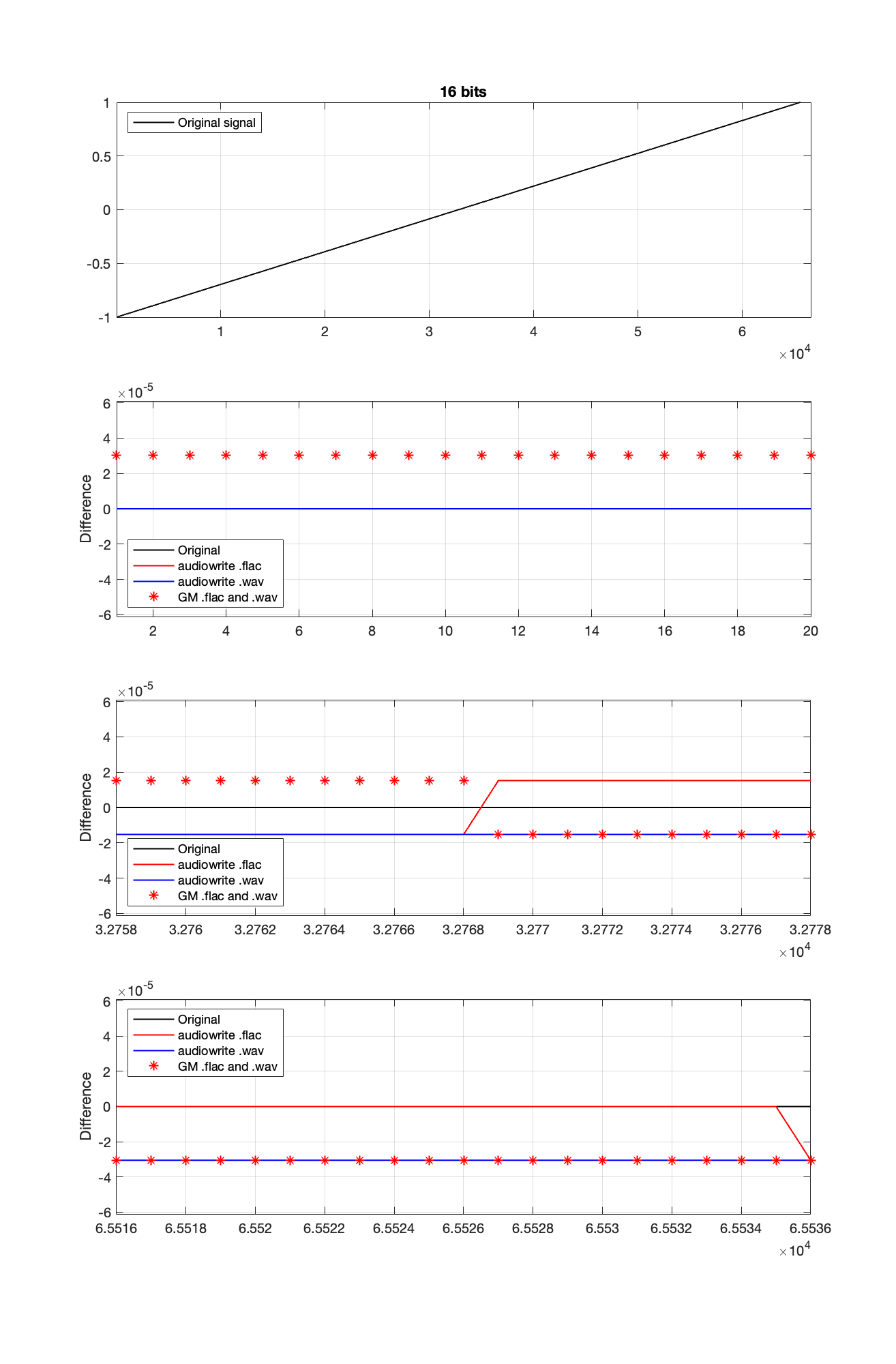
So, I go back to the ramp shown in Figure 2 and dig into the details again, zooming in on the samples near a value of -1, 0, and 1. These are shown below in Figure 4.
Figure 4.
It’s a bit cryptic to see the results in Figure 4, but let’s walk through it.
The top plot shows the ramp signal that I encoded as a 16-bit audio file in 4 different ways: as a .wav and a .flac, using audiowrite’s quantiser and mine.
The second plot shows the differences in the imported files relative to the original for the first 20 samples, which correspond to the bottom 20 quantisation levels. As can be seen there, the audiowrite quantiser’s result appears to be identical to the original (they’re not, as we saw in the middle plot of Figure 1, but they’re close…). My quantiser is one level higher. This is because I’m scaling my original signal so that it can’t reach the bottom, as I talked about in Part 2.
The third plot shows the behaviour of the three quantisers (2 audiowrites and mine) around the 0 value ±10 quantisation levels. Note that there’s no sample with a value of 0 (Because two’s complement is not symmetrical around the 0 value.). It’s not immediately obvious there, but all three quantisers have an “error” of 1/2 a quantisation level step around 0.
Below 0, both of audiowrite’s quantisers have a negative offset, and mine has a positive offset.
Above 0, audiowrite’s .flac quantiser has a positive offset whereas both audiowrite’s .wav quantiser and mine have a negative offset
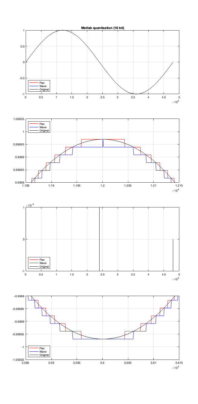
If the signal were a sine wave, then we’d see the same thing, it would just be harder to interpret, as shown in Figure 5. (There’s nothing useful shown in the third plot there because when you zoom in so closely , the slope of the sine wave as it passes 0 is really steep…)
Figure 5.
I titled this series of posts “Excruciating minutiae” for a reason. The “error” (let’s call it a “difference” instead) is VERY small. It’s a difference of 1 quantisation level on a portion of the signal, which raises the very pragmatic question: “So what?”
Unless you’re REALLY digging into the bottom of the noise floor of a device, you probably never need to care about this. (In fact, even if you ARE digging into the bottom of the noise floor, you might not need to care.)
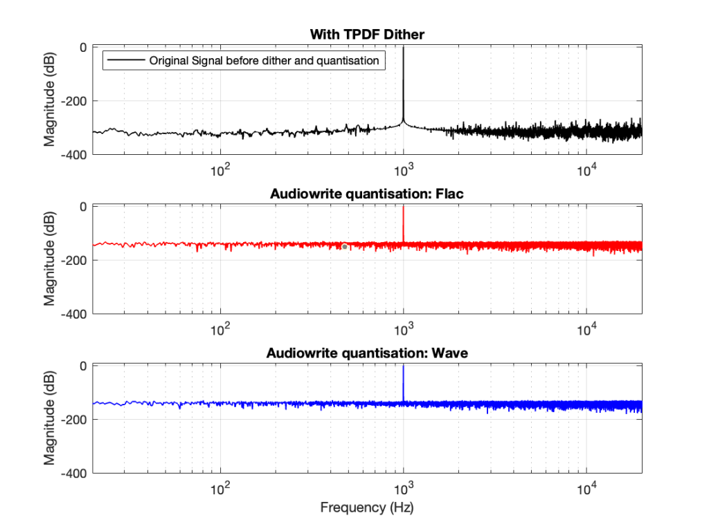
You CERTAINLY don’t have to worry about it if you’re just writing audio files to listen to, since you should be dithering those with TPDF dither, which will create a noise floor that is FAR above the “errors” caused by the differences I described above. This can be seen in Figures 6 and 7 below.
Figure 6
Figure 7
In other words, I’ve been using Matlab to export test files both in .wav and .flac for at least 20 years, and it’s only now that I’ve noticed this issue, which is another way of saying “don’t worry about it…”
Nota Bene
If you’re still awake, you might notice that there is one loose end… At the top of this posting I said
The less-important (but more interesting, later…) thing is that, for the FLAC import, every odd-numbered FFT bin is -∞ dB, which means that there is absolutely NO energy at those frequencies.
That will be the topic of another posting, since it’s more or less unrelated to this one – it was just an artefact of the test I described above.
In Part 2 of this series, I wrote the following sentence:
The easiest (and possibly best) way to do this is to create white noise with a triangular probability distribution function and a peak-to-peak amplitude of ± 1 quantisation level.
That’s a very busy sentence, so let’s unpack it a little.
Rolling the dice
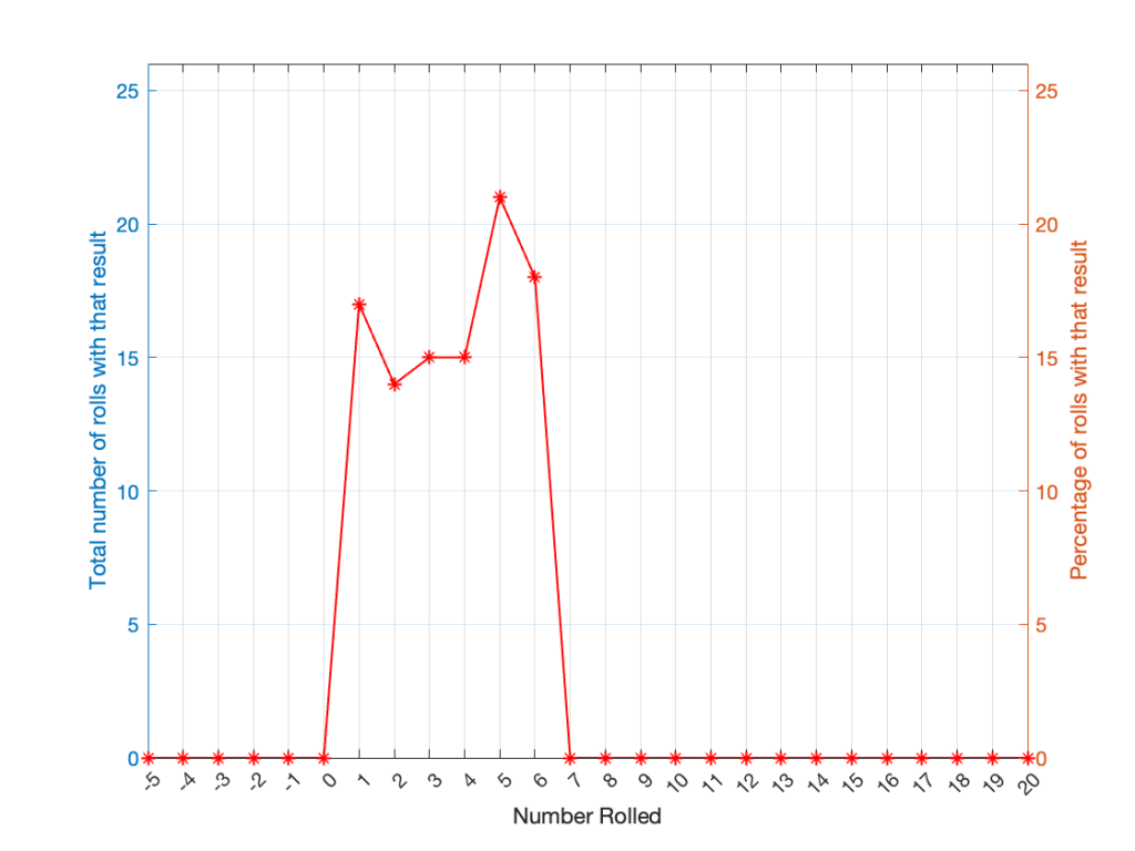
If you roll one die, you have an equal probability of rolling any number between 1 and 6 (inclusive). Let’s roll one die 100 times counting the number of times we get a 1, or a 2, or a 3, and so on up to 6.
Number rolled
Number of times the number was rolled
Percentage of times the number was rolled
1
17
17
2
14
14
3
15
15
4
15
15
5
21
21
6
18
18
(Note that the percentage of times each number was rolled is the same as the number of times each number was rolled only because I rolled the die 100 times.)
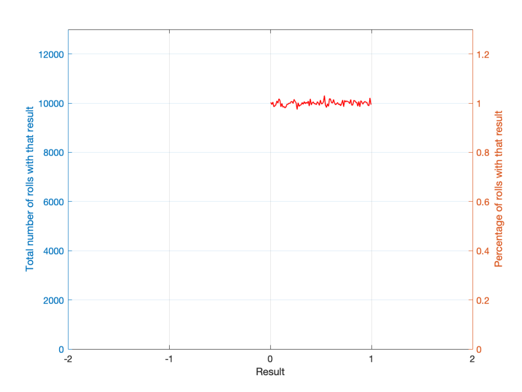
If I plot those results, it looks like Figure 1.
Figure 1. The results of rolling 1 die 100 times.
It may be weird, but I’ve plotted the number of times I rolled -5 or 13 (for example). These are 0 times because it’s impossible to get those numbers by rolling one die. But the reason I put those results in there will make more sense later.
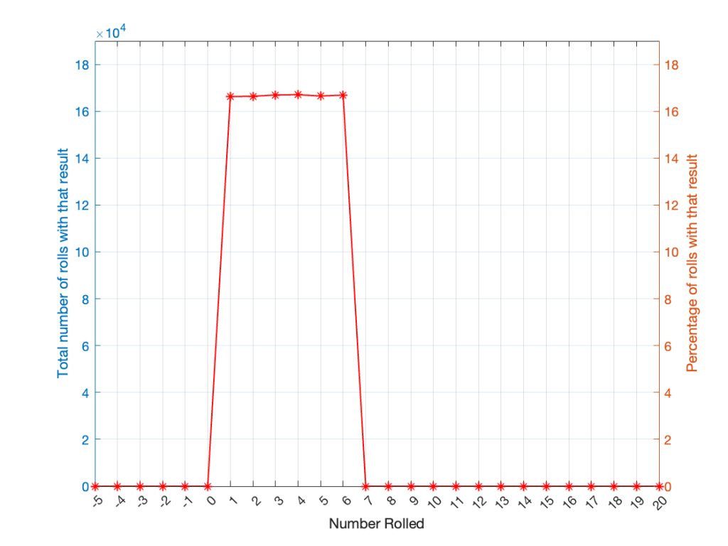
Let’s keep rolling the die. If I do it 1,000,000 times instead of 100, I get these results:
ed
Number of times the number was rolled
Percentage of times the number was rolled
1
166225
16.6225
2
166400
16.6400
3
166930
16.6930
4
167055
16.7055
5
166501
16.6501
6
166889
16.6889
Now, since I rolled many, many, more times, it’s more obvious that the six results have an equal probability. The more I roll the die, the more those numbers get closer and closer to each other.
Figure 2.
Take a look at the shape of the plot above. The area under the line from 1 to 6 (inclusive) is almost a rectangle because the six numbers are all almost the same.
The shape of that plot shows us the probability of rolling the six numbers on the die, so we call it a probability density function or PDF. In this case, we see a rectangular PDF.
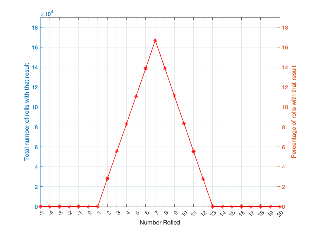
But what happens if we roll two dice instead? Now things get a little more complicated, since there is more than one way to get a total result, as shown in the table below.
Total
2
1+1
3
1+2
2+1
4
1+3
2+2
3+1
5
1+4
2+3
3+2
4+1
6
1+5
2+4
3+3
4+2
5+1
7
1+6
2+5
3+4
4+3
5+2
6+1
8
2+6
3+5
4+4
5+3
6+2
9
3+6
4+5
5+4
6+3
10
4+6
5+5
6+4
11
5+6
6+5
12
6+6
As can be (hopefully) seen in the table, there is only one way to roll a 2, and there’s only one way to roll a 12. But there are 6 different ways to roll a 7. Therefore, if you’re rolling two dice, it’s 6 times more likely that you’ll roll a 7 than a 12, for example.
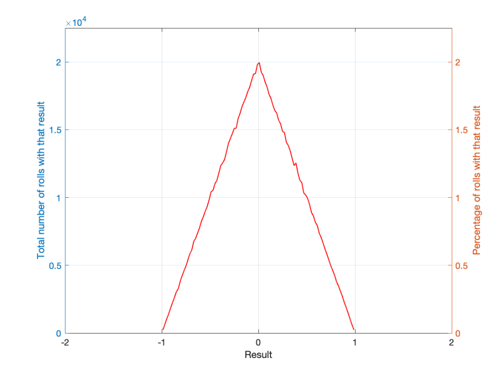
If I were to roll two dice 1,000,000 times, I would get a PDF like the one shown in Figure 3.
Figure 3.
I won’t explain why this would be considered to be a triangular PDF.
Whether you roll one die or two dice, the number you get is random. In other words, you can’t use the past results to predict what the next number will be. However, if you are rolling one die, and you bet that you’ll roll a 6 every time, you’ll be right about 16.7% of the time. If you’re rolling two dice and you bet that you’ll roll a 12 every time, you’ll only be right about 2.8% of the time.
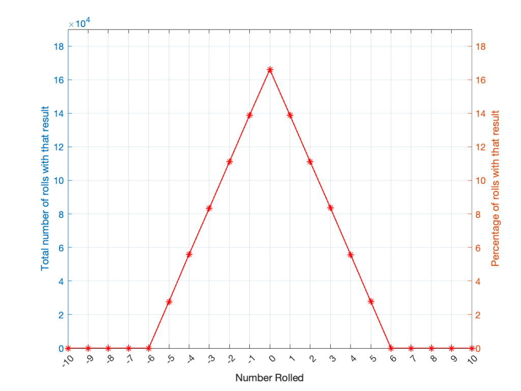
Let’s take two dice of different colours, say, one red die and one blue die. We’ll roll both dice again, but instead of adding the two values, we’ll subtract the blue value from the red one. If we do this 1,000,000 times, we’ll get something like the results shown below in Figure 4.
Figure 4.
Notice that the probability density function keeps the same shape, it’s just moved down to a range of ±5 instead of 2 to 12.
Generating noise
In audio, noise is a sound that is completely random. In other words, just like the example with the dice, in a digital audio signal, you can’t predict what the next sample value will be based on the past sample values. However, there are many different ways of generating that random number and manipulating its characteristics.
Let’s start with a computer algorithm that can generate a random number between 0 and 1 (inclusive) with a rectangular PDF. We’ll then ask the algorithm to spit out 1,000,000 values. If the numbers really are random, and the computer has infinite precision, then we’ll probably get 1,000,000 different numbers. However, we’re not really interested in the numbers themselves – we’re interested in how they’re distributed between 0.00 and 1.00. Let’s say we divide up that range into 100 steps (or “buckets”) that are 0.01 wide and count how many of our random numbers fall into each group. So, we’ll count how many are between 0.0 and 0.01, between 0.01 and 0.02, and so on up to 0.99 to 1.00. We’ll get something like Figure 5.
Figure 5.
I’ve only plotted the probabilities of the possible values: 0 to 1, which winds up showing only the top of the rectangle in the rectangular PDF.
If I generate 1,000,000 random numbers with that algorithm, and then subtract 1,000,000 other random numbers, one by one, and find the probabilities of the result, the answer will be familiar.
Figure 6.
So, this is how we make the noise that’s added to the signal. If, for each sample, you generate two random numbers (making sure that your algorithm has a rectangular PDF) and subtract one from the other, you have the dither signal that will have a maximum level of ±1 quantisation level.
The signal (with a maximum range of ±1) is scaled up by multiplying it by 2(NumberOfBits-1)-2
then you add the result of the dither generator
then the total is rounded to the nearest integer value
and then the result is scaled back down by a factor of 2(NumberOfBits-1) to bring its back down to a range of ±1 to get it ready for exporting to a standard audio file format like .wav or .flac.
In other words, assuming that you have an audio signal called “Signal” that has a range of ±1 and consists of floating point values:
A question came to my desk this week from a customer who would like to connect a third-party streaming device to his Beolab 50s. He plans to use a USB-Audio connection and his question was “Should I control the volume of the audio signal in the streamer or in the Beolab 50s?” There are three different ways to configure these two options:
Control the volume in the streamer using its interface, and send a signal that has been volume-regulated to the Beolab 50s, which should then be set to have a start up default volume such that the maximum volume on the streamer results in a level that is as loud as the customer will ever want it to be. In order to do this, the Beolab 50s need to be set to ignore the volume information that is received on the USB-Audio connection.
Set the streamer to output an unregulated signal, and set the Beolab 50s to obey the volume information that is received on the USB-Audio connection, then use the streamer’s interface for the volume control (which would actually be happening inside the Beolab 50s).
Set the streamer to output an unregulated signal, and set the Beolab 50s to disobey the volume information that is received on the USB-Audio connection, then use the Beolab 50’s interface for the volume control (which would actually be happening inside the Beolab 50s).
Of course, one way to answer the question is “where do you want to control the volume?” For example, if it’s with a remote control for the Beolab 50s, then the answer is “use option #3”. If you’d prefer to use the streamer’s app, for example, then the answer is “use option #1 or #2”.
However, the question came to my desk because it was specifically about the technical performance of the audio signal. Which of these three options results in the highest audio “quality”? (I put the word “quality” in quotation marks because it is a loaded term, and might mean different things to different persons…)
The simplest answer without getting into any details is “it probably doesn’t matter“. However, that answer is based on a couple of assumptions that may or may not be wrong.
Hypothetically, the Beolab 50 can output an audio signal that peaks at about 122 dB SPL measured at 1 m in a free field, albeit not at all frequencies present at its output. (This is because there are some physical limitations of how far the woofers can move, which means that you can’t get 122 dB SPL at 20 Hz, for example.) The noise floor of the Beolab 50s is about 0 dB SPL measured in the same place (again, this is frequency-dependent). So, it has a total dynamic range at its output of about 122 dB.
The maximum output level is a result of a combination of the loudspeaker drivers, the amplifiers, and the power supply, however, these have all been chosen to reach their maximum outputs approximately simultaneously, so changing one of the three won’t make a big difference.
The noise floor is a result of the combination of the loudspeaker drivers’ sensitivities, the amplifiers’ noise floors, and the signal that feeds the amplifiers: the DAC outputs’ noise floors. For the purposes of this discussion, I’m sticking with a digital input, so we don’t need to worry about the noise floor of the ADC at the loudspeaker’s input.
If you have an audio signal at one of the digital inputs of the Beolab 50, and that signal is at its loudest possible level (for a sine wave, that’s 0 dB FS; or 0 dB relative to Full Scale). At Beolab 50’s maximum volume setting, this will produce a peak output level of 122 dB SPL (depending on the frequency as I mentioned above).
All digital inputs of the Beolab 50 accept at least a 24 bit word length. This means that the dynamic range of the digital input signal itself is about 6 * 24 – 3 = 141 dB. This in turn means that the hypothetical noise floor of a correctly-dithered 24-bit signal is 19 dB below the noise floor of the loudspeakers even at their maximum volume setting. (because 122 – 141 = -19)
In other words, if we assume that the streamer has a correctly-implemented gain function for its volume control, using TPDF dither implemented at the 24-bit level, then its noise floor will be 19 dB below the “natural” noise floor of the Beolab 50. Therefore, if the volume is controlled in the streamer, any artefacts will be masked by the 50s themselves.
On the other hand, the Beolab 50s volume control is done using a gain function that is performed in a 32-bit floating point calculation, which means that it has a dynamic range of 144 to 150 dB. (See this posting for an explanation and comparison of fixed point and floating point systems.) So the noise generated by the internal volume control will be somewhere between 22 and 26 dB below the “natural” noise floor of the Beolab 50.
So, (assuming my assumptions are correct) the noise floor that is produced by controlling the volume control in either the streamer or the Beolab 50s is FAR below the constant noise floor of the DAC / amplifiers.
In addition, the noise floors have roughly the same spectra (in other words, you don’t have pink noise in one case but white noise in the other; they’re all producing white noise). And since both are so far below, it really doesn’t matter. Arguing about whether the noise is 19 dB lower or 22 dB lower is a waste of good argument time, unless you paid for the four-and-a-half-hour argument instead of the five-minute one…
Important Notes
If the customer was asking about using the analogue input, then the answer MIGHT have been different.
Also, if my assumption about a 24-bit signal coming from the streamer, or that it has a correctly-implemented gain function for its volume control are incorrect, the this answer MIGHT be incorrect as well.
In Part 1 of this series, I talked about how a binaural audio signal can (hypothetically, with HRTFs that match your personal ones) be used to simulate the sound of a source (like a loudspeaker, for example) in space. However, to work, you have to make sure that the left and right ears get completely isolated signals (using earphones, for example).
In Part 2, I showed how, with enough processing power, a large amount of luck (using HRTFs that match your personal ones PLUS the promise that you’re in exactly the correct location), and a room that has no walls, floor or ceiling, you can get a pair of loudspeakers to behave like a pair of headphones using crosstalk cancellation.
There’s not much left to do to create a virtual loudspeaker. All we need to do is to:
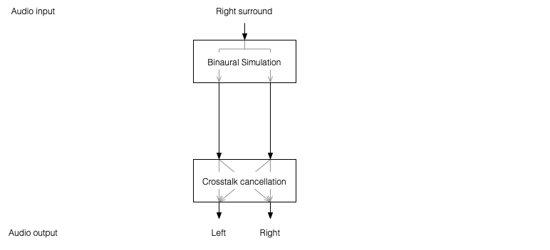
Take the signal that should be sent to a right surround loudspeaker (for example) and filter it using the HRTFs that correspond to a sound source in the location that this loudspeaker would be in. REMEMBER that this signal has to get to your two ears since you would have used your two ears to hear an actual loudspeaker in that location.
Send those two signals through a crosstalk cancellation processing system that causes your two loudspeakers to behave more like a pair of headphones.
Figure 1: A block diagram of the system described above.
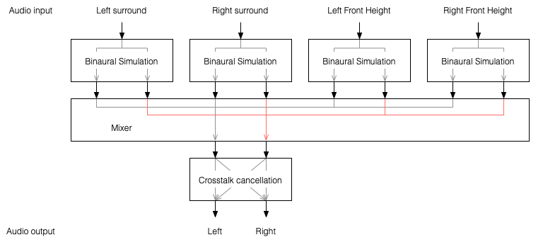
One nice thing about this system is that the crosstalk cancellation is only there to ensure that the actual loudspeakers behave more like headphones. So, if you want to create more virtual channels, you don’t need to duplicate the crosstalk cancellation processor. You only need to create the binaurally-processed versions of each input signal and mix those together before sending the total result to the crosstalk cancellation processor, as shown below.
Figure 2: You only need one crosstalk cancellation system for any number of virtual channels.
This is good because it saves on processing power.
So, there are some important things to realise after having read this series:
All “virtual” loudspeakers’ signals are actually produced by the left and right loudspeakers in the system. In the case of the Beosound Theatre, these are the Left and Right Front-firing outputs.
Any single virtual loudspeaker (for example, the Left Surround) requires BOTH output channels to produce sound.
If the delays (aka Speaker Distance) and gains (aka Speaker Levels) of the REAL outputs are incorrect at the listening position, then the crosstalk cancellation will not work and the virtual loudspeaker simulation system won’t work. How badly is doesn’t work depends on how wrong the delays and gains are.
The virtual loudspeaker effect will be experienced differently by different persons because it’s depending on how closely your actual personal HRTFs match those predicted in the processor. So, don’t get into fights with your friends on the sofa about where you hear the helicopter…
The listening room’s acoustical behaviour will also have an effect on the crosstalk cancellation. For example, strong early reflections will “infect” the signals at the listening position and may/will cause the cancellation to not work as well. So, the results will vary not only with changes in rooms but also speaker locations.
Finally, it’s worth nothing that, in the specific case of the Beosound Theatre, by setting the Speaker Distances and Speaker Levels for the Left and Right Front-firing outputs for your listening position, then you have automatically calibrated the virtual outputs. This is because the Speaker Distances and Speaker Levels are compensations for the ACTUAL outputs of the system, which are the ones producing the signal that simulate the virtual loudspeakers. This is the reason why the four virtual loudspeakers do not have individual Speaker Distances and Speaker Levels. If they did, they would have to be identical to the Left and Right Front-firing outputs’ values.
In Part 1, I talked at how a binaural recording is made, and I also mentioned that the spatial effects may or may not work well for you for a number of different reasons.
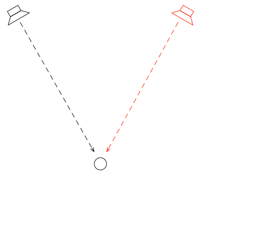
Let’s go back to the free field with a single “perfect” microphone to measure what’s happening, but this time, we’ll send sound out of two identical “perfect” loudspeakers. The distances from the loudspeakers to the microphone are identical. The only difference in this hypothetical world is that the two loudspeakers are in different positions (measuring as a rotational angle) as shown in Figure 1.
Figure 1: Two identical, “perfect” loudspeakers in a free field with a single “perfect” microphone.
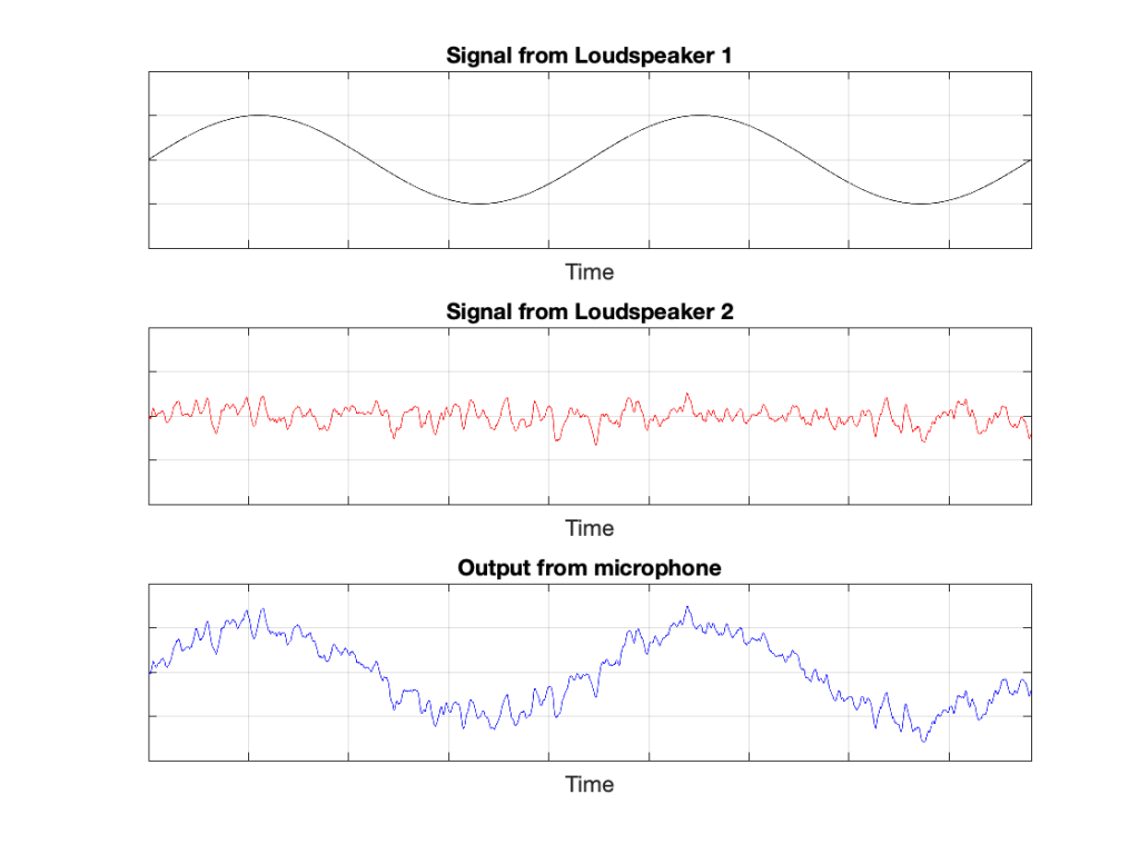
In this example, because everything is perfect, and the space is a free field, then output of the microphone will be the sum of the outputs of the two loudspeakers. (In the same way that if your dog and your cat are both asking for dinner simultaneously, you’ll hear dog+cat and have to decide which is more annoying and therefore gets fed first…)
Figure 2: The output from the microphone is the sum of the outputs from the two loudspeakers. At any moment in time, the value of the top plot + the value of the middle plot = the value of the bottom plot.
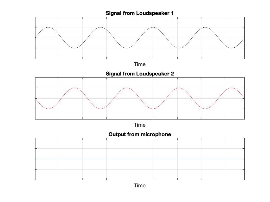
IF the system is perfect as I described above, then we can play some tricks that could be useful. For example, since the output of the microphone is the sum of the outputs of the two loudspeakers, what happens if the output of one loudspeaker is identical to the other loudspeaker, but reversed in polarity?
Figure 3: If the output of Loudspeaker 1 is exactly the same as the output of Loudspeaker 2 except for polarity, then the sum (the output of the microphone) is always 0.
In this example, we’re manipulating the signals so that, when they add together, you nothing at the output. This is because, at any moment in time, the value of Loudspeaker 2’s output is the value of Loudspeaker 1’s output * -1. So, in other words, we’re just subtracting the signal from itself at the microphone and we get something called “perfect cancellation” because the two signals cancel each other at all times.
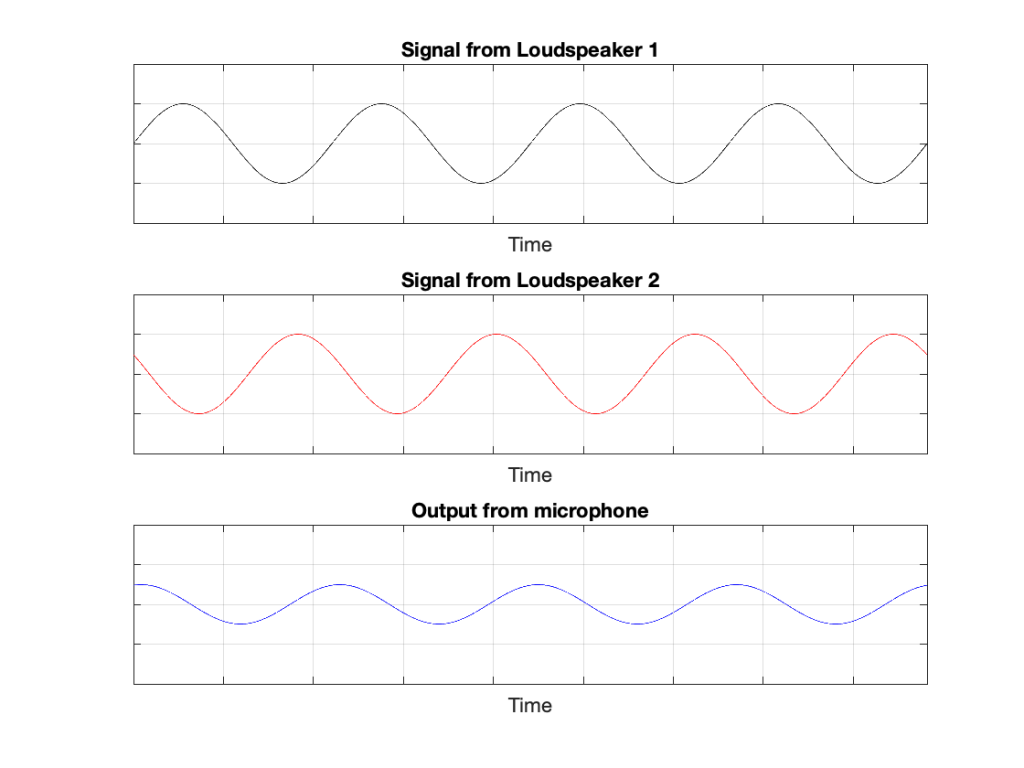
Of course, if anything changes, then this perfect cancellation won’t work. For example, if one of the loudspeakers moves a little farther away than the other, then the system is broken, as shown below.
Figure 4: A small shift in time in the output of Loudspeaker 2 cases the cancellation to stop working so well.
Again, everything that I’ve said above only works when everything is perfect, and the loudspeakers and the microphone are in a free field; so there are no reflections coming in and ruining everything.
We can now combine these two concepts:
using binaural signals to simulate a sound source in a location (although this would normally be done using playback over earphones to keep it simple) and
using signals from loudspeakers to cancel each other at some location in space as a
to create a system for making virtual loudspeakers.
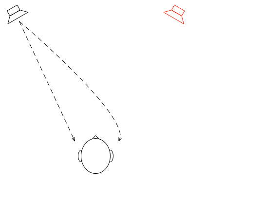
Let’s suspend our adherence to reality and continue with this hypothetical world where everything works as we want… We’ll replace the microphone with a person and consider what happens. To start, let’s just think about the output of the left loudspeaker.
Figure 5: The output of the left loudspeaker reaches both ears with different time/frequency characteristics caused by the HRTF associated with that sound source location.
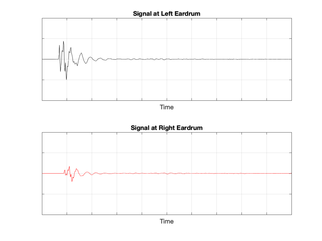
If we plot the impulse responses at the two ears (the “click” sound from the loudspeaker after it’s been modified by the HRTFs for that loudspeaker location), they’ll look like this:
Figure 6: The impulse responses of the HRTFs for a sound source at 30º left of centre.
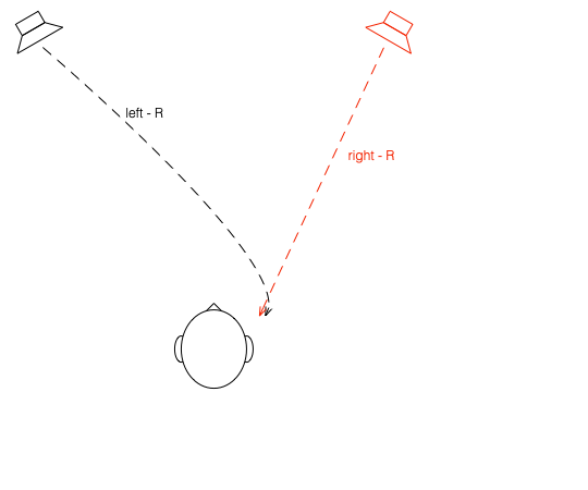
What if were were able to send a signal out of the right loudspeaker so that it cancels the signal from the left loudspeaker at the location of the right eardrum?
Figure 7: What if we could cancel the signal from the left loudspeaker at the right ear using the right loudspeaker?
Unfortunately, this is not quite as easy as it sounds, since the HRTF of the right loudspeaker at the right ear is also in the picture, so we have to be a bit clever about this.
So, in order for this to work we:
Send a signal out of the left loudspeaker. We know that this will get to the right eardrum after it’s been messed up by the HRTF. This is what we want to cancel…
…so we take that same signal, and
filter it with the inverse of the HRTF of the right loudspeaker (to undo the effects of the HRTF of the right loudspeaker’s signal at the right ear)
filter that with the HRTF of the left loudspeaker at the right ear (to match the filtering that’s done by your head and pinna)
multiply by -1 (so that it will cancel when everything comes together at your right eardrum)
and send it out the right loudspeaker.
Hypothetically, that signal (from the right loudspeaker) will reach your right eardrum at the same time as the unprocessed signal from the left loudspeaker and the two will cancel each other, just like the simple example shown in Figure 3. This effect is called crosstalk cancellation, because we use the signal from one loudspeaker to cancel the sound from the other loudspeaker that crosses to the wrong side of your head.
This then means that we have started to build a system where the output of the left loudspeaker is heard ONLY in your left ear. Of course, it’s not perfect because that cancellation signal that I sent out of the right loudspeaker gets to the left ear a little later, so we have to cancel the cancellation signal using the left loudspeaker, and back and forth forever.
If, at the same time, we’re doing the same thing for the other channel, then we’ve built a system where you have the left loudspeaker’s signal in the left ear and the right loudspeaker’s signal in the right ear; just like a pair of headphones!
However, if you get any of these elements wrong, the system will start to under-perform. For example, if the HRTFs that I use to predict your HRTFs are incorrect, then it won’t work as well. Or, if things aren’t time-aligned correctly (because you moved) then the cancellation won’t work.