Tonearm tracking error and distortion

In the last posting, I reviewed the math for calculating the tracking error for a radial tonearm. The question associated with this is “who cares?”

In the March, 1945 issue of Electronics Magazine, Benjamin Bauer supplied the answer. An error in the tracking angle results in a distortion of the audio signal. (This was also discussed in a 3-part article by Dr. John D. Seagrave in Audiocraft Magazine in December 1956, January 1957, and August 1957)

If the signal is a sine wave, then the distortion is almost entirely 2nd-order (meaning that you get the sine wave fundamental, plus one octave above it). If the signal is not a sine wave, then things are more complicated, so I will not discuss this.

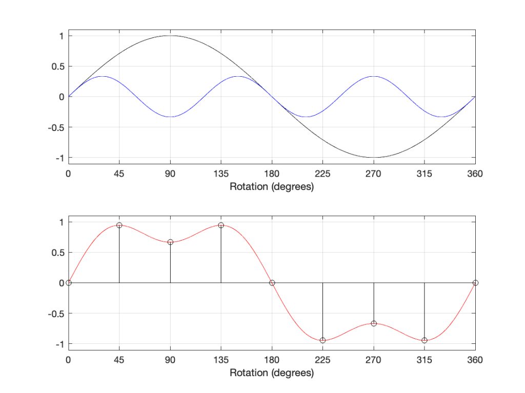
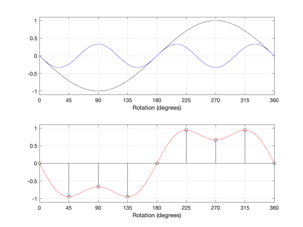
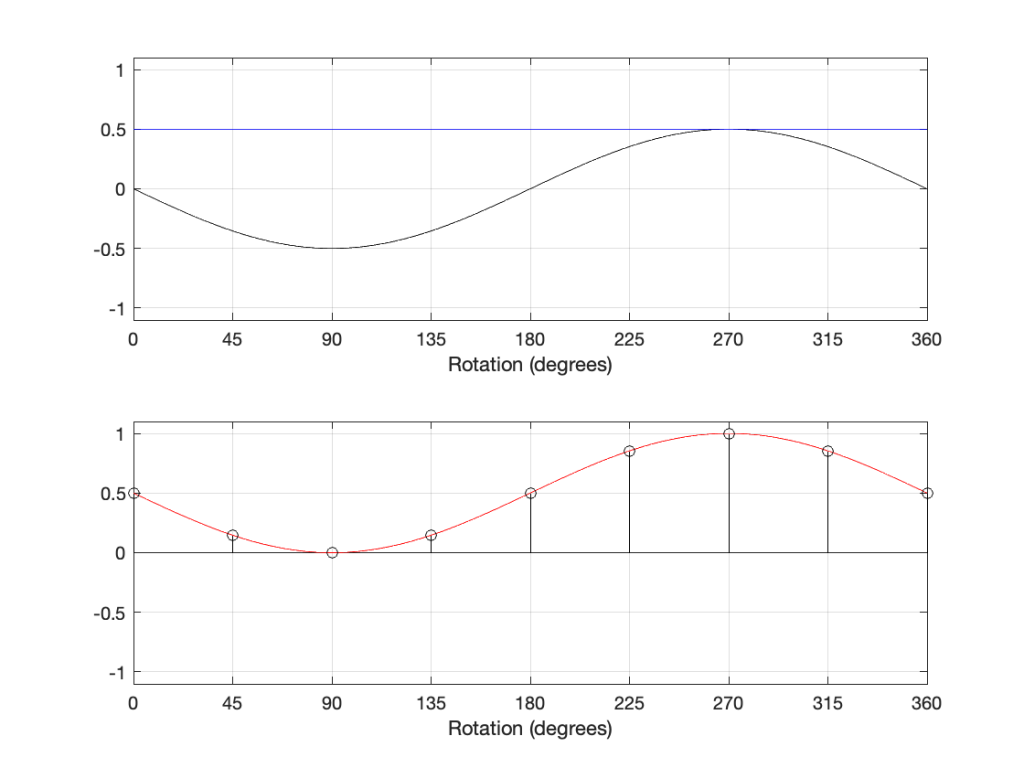
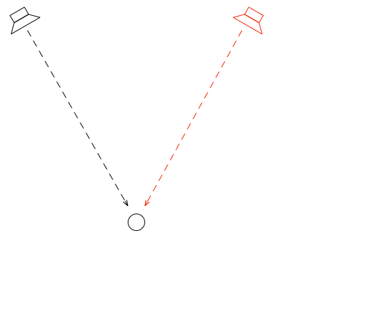
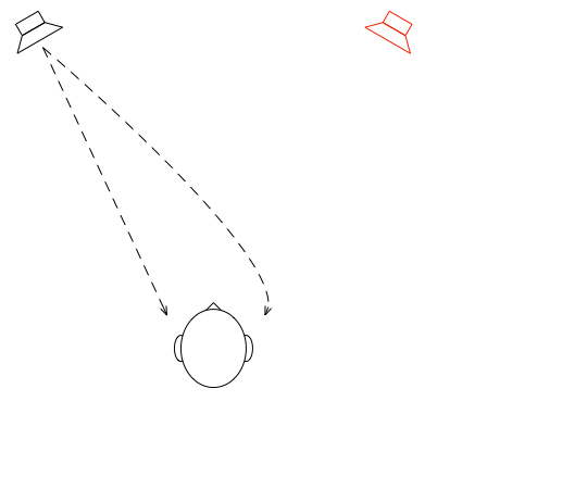
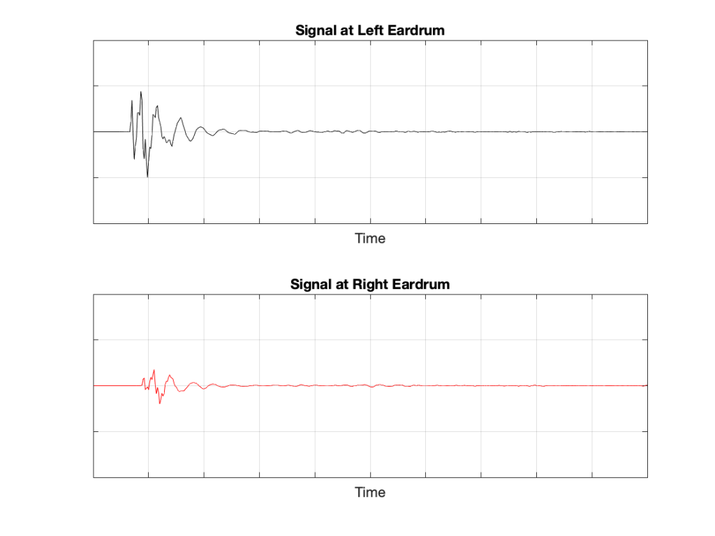
Let’s take a quick look at how the signal is distorted. An example of this is shown below.

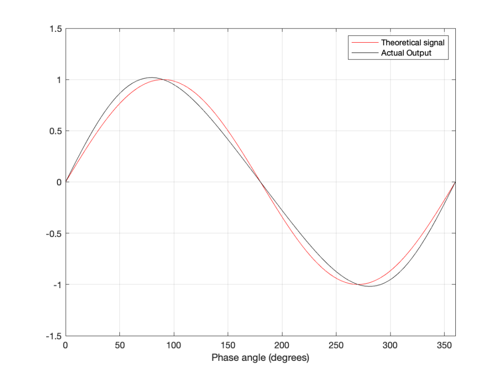
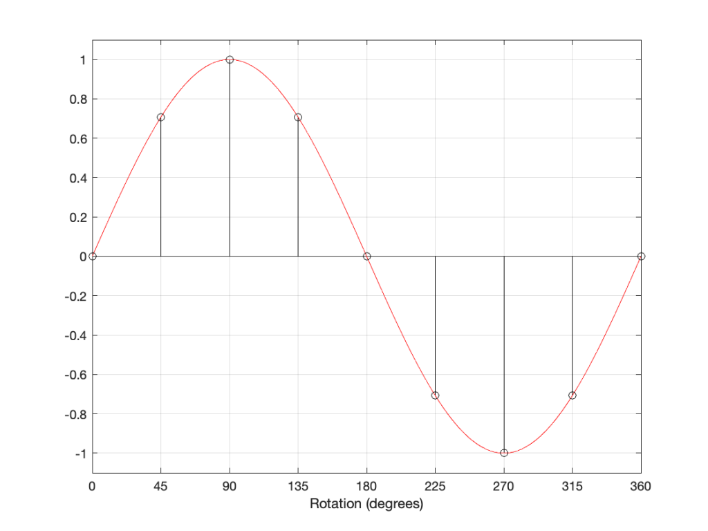
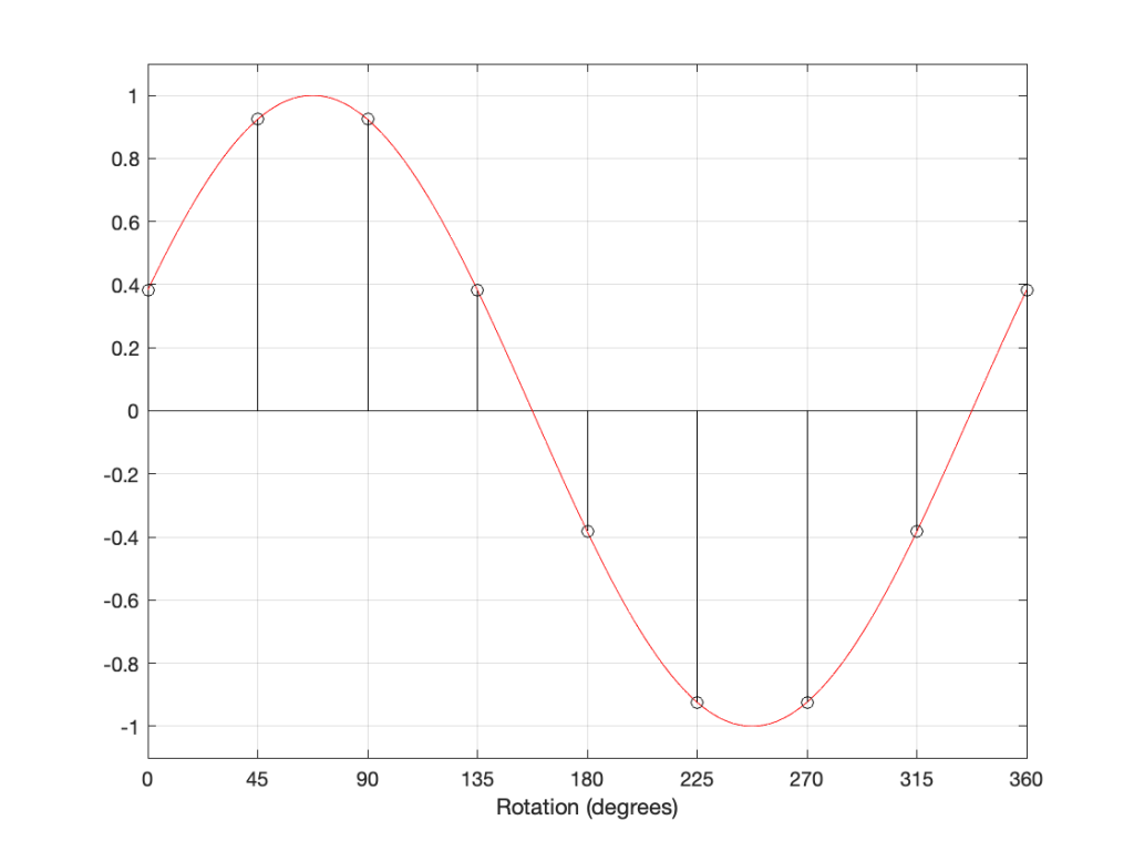
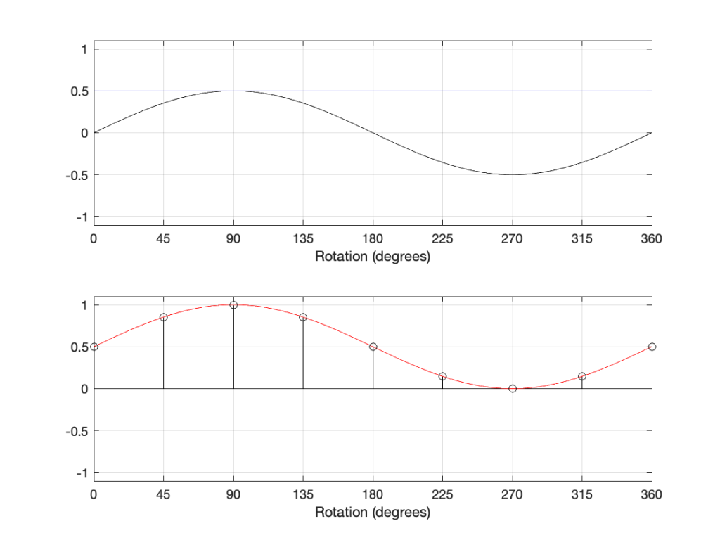
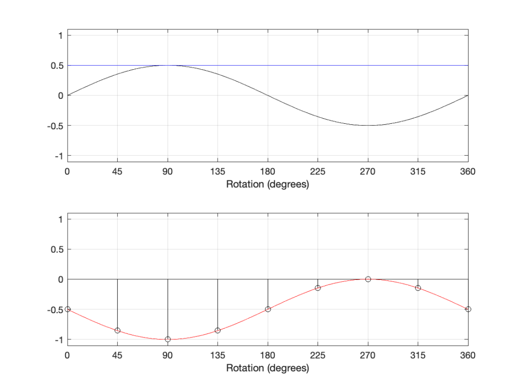
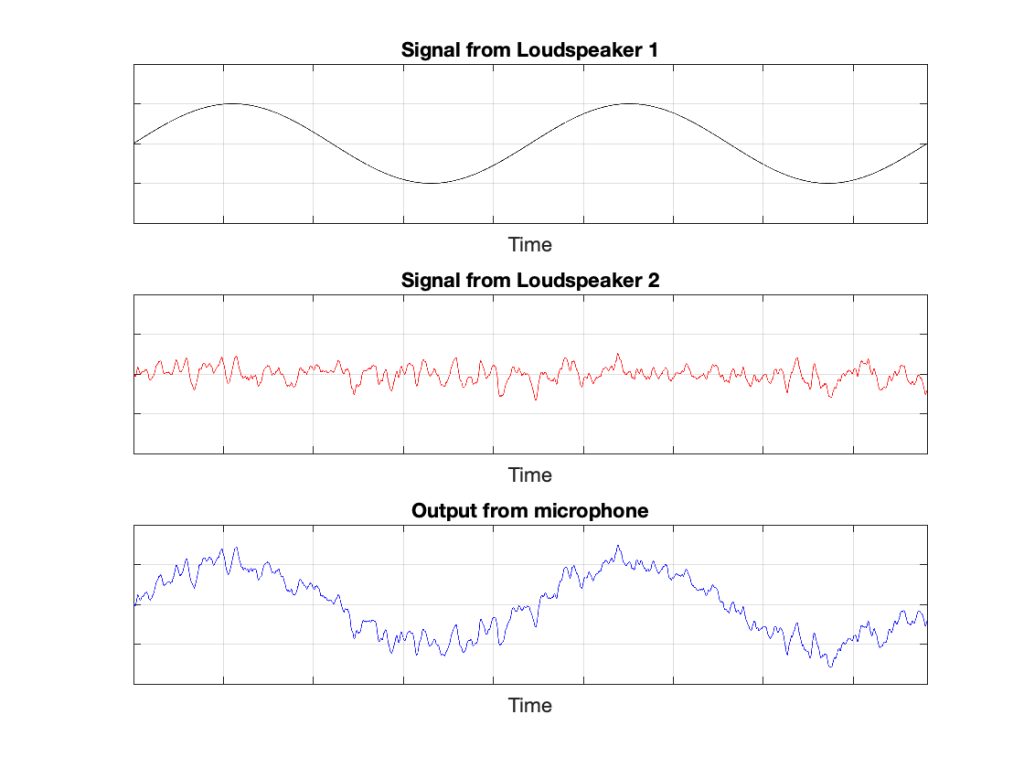
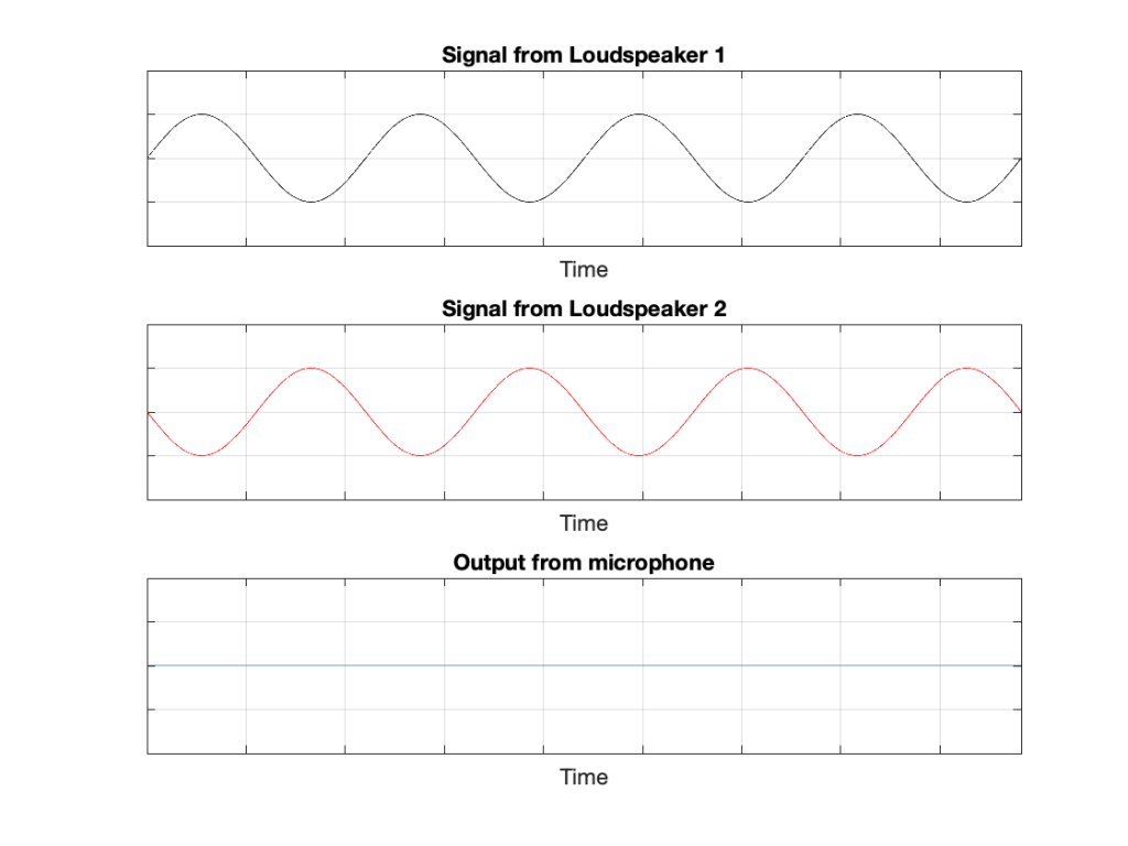
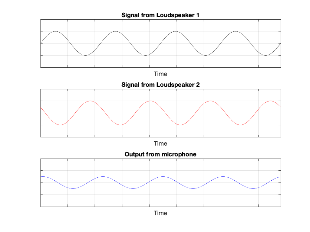
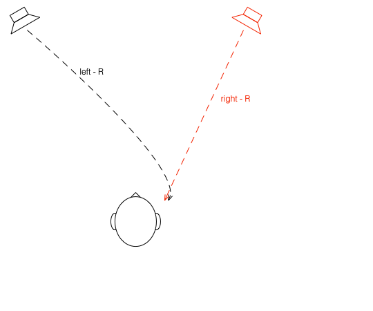
In that plot, you can see that the actual output from the stylus with a tracking error (the black curve) precedes the theoretical output that’s actually on the vinyl surface (the red curve) when the signal is positive, and lags when it’s negative. An intuitive way of thinking of this to consider the tracking error as an angular rotation, so the stylus “reads” the signal in the groove at the wrong place. This is shown below, which is merely zooming in on the figure above.

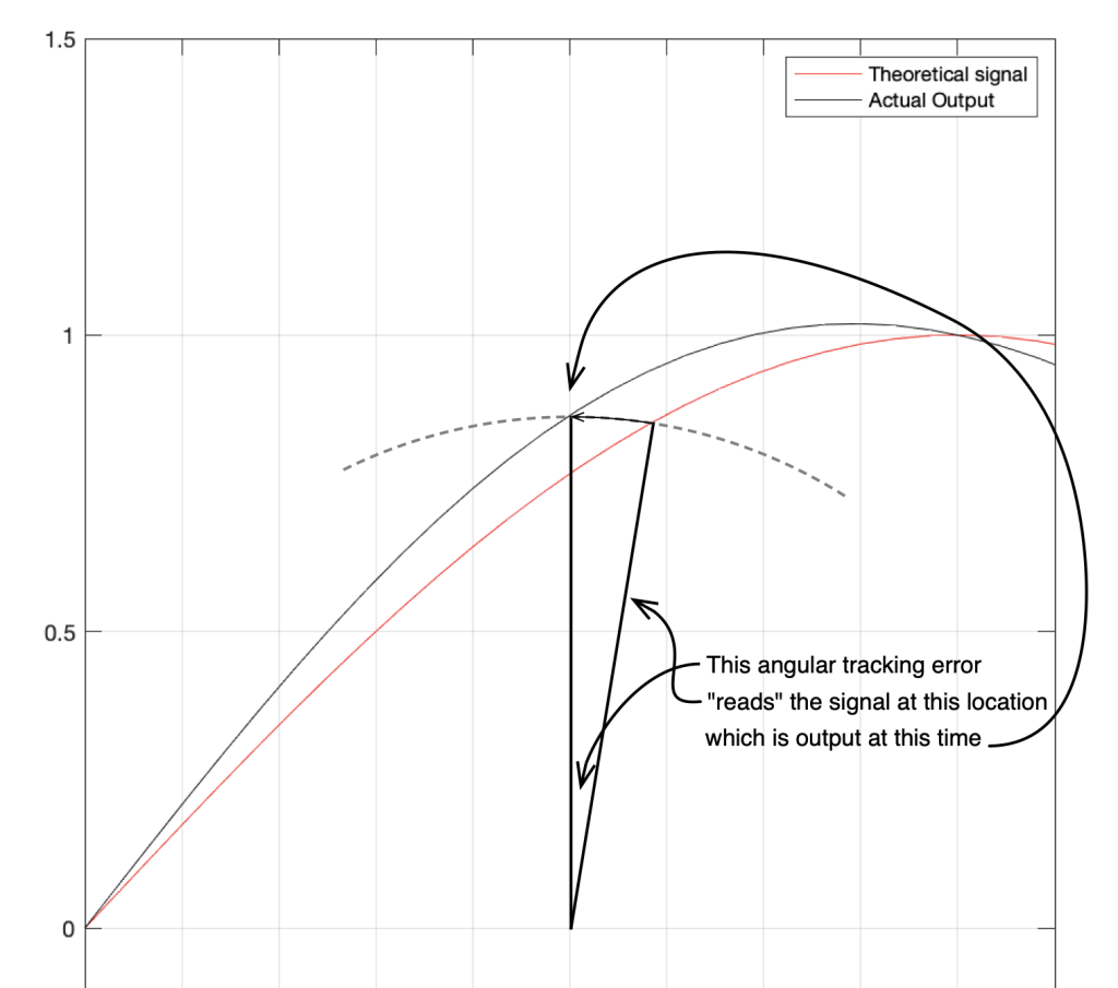
Here, you can see that the rotation (tracking error) of the stylus is getting its output from the wrong place in the groove and therefore has the wrong output at any given moment. However, the amount by which it’s wrong is dependent not only on the tracking error but the amplitude of the signal. When the signal is at 0, then the error is also 0. This is not only the reason why the distortion creates a harmonic of the sine wave, but it also explains why (as we’ll see below) the level of distortion is dependent on the level of the signal.

This intuitive explanation is helpful, but life is unfortunately, more complicated. This is because (as we saw in the previous posting), the tracking error is not constant; it changes according to where the stylus is on the surface of the vinyl.

If you dig into Bauer’s article, you’ll find a bunch of equations to help you calculate how bad things get. There are some minor hurdles to overcome, however. Since he was writing in the USA in 1945, his reference was 78 RPM records and his examples are all in inches. However, if you spend some time, you can convert this to something more useful. Or, you could just trust me and use the information below.

In the case of a sinusoidal signal the level of the 2nd harmonic distortion (in percent) can be calculated with the following equation:

PercentDistortion = 100 * (ω Αpeak α) / (ωr r)

where

  • ω is 2 * pi * the audio frequency in Hz
  • Apeak is the peak amplitude of the modulation (the “height” of the groove) in mm
  • α is the tracking error in radians
  • ωr is the rotational speed of the record in radians per second, calculated using 2 * pi * (RPM / 60)
  • r is the radius of the groove; the distance from the centre spindle to the stylus in mm

Let’s invent a case where you have a constant tracking error of 1º, with a rotational speed of 33 1/3 RPM, and a frequency of 1 kHz. Even though the tracking error remains constant, the signal’s distortion will change as the needle moves across the surface of the record because the wavelength of the signal on the vinyl surface changes (the rotational speed is the same, but the circumference is bigger at the outside edge of the record than the inside edge). The amount of error increases as the wavelength gets smaller, so the distortion is worse as you get closer to the centre of the record. This can be see in the shapes of the curves in the plot below. (Remember that, as you play the record, the needle is moving from right to left in those plots.)

You can also see in those plots that the percentage of distortion changes significantly with the amplitude of the signal. In this case, I’ve calculated using three different modulation velocities. The middle plot is 35.4 mm / sec, which is a typical accepted standard reference level, which we’ll call 0 dB. The other two plots have modulation velocities of -3 dB (25 mm / sec) and + 3 dB (50 mm / sec).

Sidebar: If you want to calculate the Amplitude of the modulation

Apeak = (ModulationVelocity * sqrt(2)) / (2 * pi * FrequencyInHz)

Note that this simplifies the equation for calculating the distortion somewhat.

Also, if you need to convert radians to degrees, then you can multiply by 180/pi. (about 57.3)

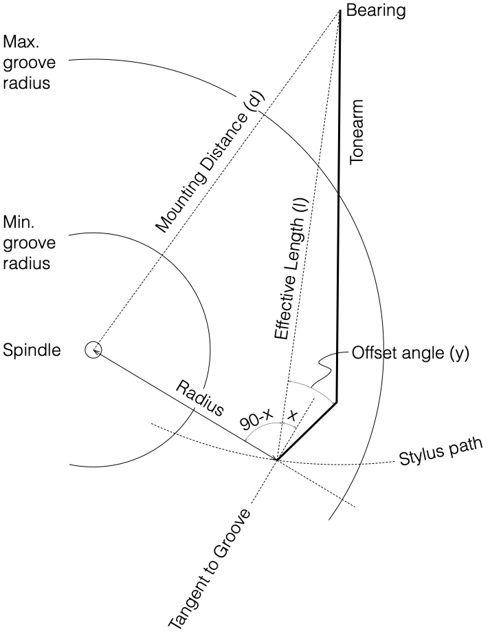
Of course, unless you have a very badly-constructed linear tracking turntable, you will never have a constant tracking error. The tracking error of a radial tonearm is a little more complicated. Using the recommended values for the “well known tonearm” that I used in the last posting:

  • Effective Length (l) : 233.20 mm
  • Mounting Distance (d) : 215.50 mm
  • Offset angle (y) : 23.63º

and assuming that this was done perfectly, we get the following result for a 33 1/3 RPM album.

You can see here that the distortion drops to 0% when the tracking error is 0º, which (in this case) happens at two radii (distances between the centre spindle and the stylus).

If we do exactly the same calculation at 45 RPM, you’ll see that the distortion level drops (because the value of ωr increases), as shown below. (But good luck finding a 12″ 45 RPM record… I only have two in my collection, and one of those is a test record.)

Important notes:

Everything I’ve shown above is not to be used as proof of anything. It’s merely to provide some intuitive understanding of the relationship between radial tracking tonearms, tracking error, and the resulting distortion. There is one additional important reason why all this should be taken with a grain of salt. Remember that the math that I’ve given above is for 78 RPM records in 1945. This means that they were for laterally-modulated monophonic grooves; not modern two-channel stereophonic grooves. This means that the math above isn’t accurate for a modern turntable, since the tracking error will be 45º off-axis to the axis of modulation of the groove wall. This rotation can be built into the math as a modification applied to the variable α, however, I’m not going to complicate things further today…

In addition, the RIAA equalisation curve didn’t get standardised until 1954 (although other pre-emphasis curves were being used in the 1940s). Strictly speaking, the inclusion of a pre-emphasis curve doesn’t really affect the math above, however, in real life, this equalisation makes it a little more complicated to find out what the modulation velocity (and therefore the amplitude) of the signal is, since it adds a frequency-dependent scaling factor on things. On the down-side, RIAA pre-emphasis will increase the modulation velocity of the signal on the vinyl, resulting in an increase in the distortion effects caused by tracking error. On the up-side, the RIAA de-emphasis filtering is applied not only to the fundamentals, but the distortion components as well, so the higher the order of the unwanted harmonics, the more they’ll be attenuated by the RIAA filtering. How much these two effects negate each other could be the subject of a future posting; if I can wrap my own head around the problem…

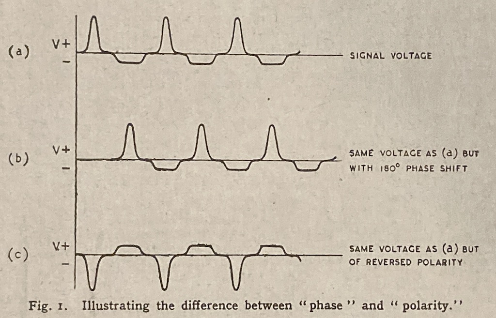
One extra comment for the truly geeky:

You may be looking at the last two plots above and being confused in the same way that I was when I made them the first time. If you look at the equation, you can see that the PercentDistortion is related to α: the tracking error. However, if you look at the plots, you’ll see that I’ve shown it as being related to | α |: the absolute value of the tracking error instead. This took me a while to deal with, since my first versions of the plots were showing a negative value for the distortion. “How can a negative tracking result in distortion being removed?” I asked myself. The answer is that it doesn’t. When the tracking error is negative, then the angle shown in the second figure above rotates counter-clockwise to the left of the vertical line. In this case, then the output of the stylus lags for positive values and precedes for negative values (opposite to the example I gave above), meaning that the 2nd-order harmonic flips in polarity. SINCE you cannot compare the phase of two sine tones that do not have the same frequency, and SINCE (for these small levels of distortion) it’ll sound the same regardless of the polarity of the 2nd-order harmonic, and SINCE (in real-life) we don’t listen to sine tones so we get higher-order THN and IMD artefacts, not just a frequency doubling, THEN I chose to simplify things and use the absolute value.
Post Script to the comment for geeks: This conclusion was confirmed by J.K. Stevenson’s article called “Pickup Arm Design” in the May, 1966 edition of Wireless World where he states “The sign of φ (positive or negative) is ignored as it has no effect on the distortion.” (He uses φ to denote the tracking error angle.)

Penultimate Post Script:

J.K. Stevenson’s article gives an alternative way of calculating the 2nd order harmonic distortion that gives the same results. However, if you are like me, then you think in modulation velocity instead of amplitude, so it’s easier to not convert on the way through. This version of the equation is

PercentDistortion = 100 * (Vpeak tan(α)) / (μ)

where

  • Vpeak is the peak modulation velocity in mm/sec
  • α is the tracking error in radians
  • μ is the groove speed of the record in mm/sec calculated using 2*pi*(rpm/60)*r
  • r is the radius of the groove; the distance from the centre spindle to the stylus in mm

Final Post-Script:

I’ve given this a lot of thought over the past couple of days and I’m pretty convinced that, since the tracking error is a rotation angle on an axis that is 45º away from the axis of modulation of the stylus (unlike the assumption that we’re dealing with a monophonic laterally-modulated groove in all of the above math), then, to find the distortion for a single channel of a stereophonic groove, you should multiply the results above by cos(45º) or 1/sqrt(2) or 0.707 – whichever you prefer. If you are convinced that this was the wrong thing to do, and you can convince me that you’re right, I’ll be happy to change it to something else.

Tonearm alignment and tracking error

The June 1980 issue of Audio Magazine contains an article written by Subir K. Pramanik called “Understanding Tonearms”. This is a must-read tutorial for anyone who is interested in the design and behaviour of radial tonearms.

One of the things Pram talked about in that article concerned the already well-known relationship between tonearm geometry, its mounting position on the turntable, and the tracking error (the angular difference between the tangent to the groove and the cantilever axis – or the rotation of the stylus with respect to the groove). Since the tracking error is partly responsible for distortion of the audio signal, the goal is to minimise it as much as possible. However, without a linear-tracking system (or an infinitely long tonearm), it’s impossible to have a tracking error of 0º across the entire surface of a vinyl record.

One thing that is mentioned in the article is that “Small errors in the mounting distance from the centre of the platter … can make comparatively large differences in angular error” So I thought that I’d do a little math to find out this relationship.

The article contains the diagram shown below, showing the information required to do the calculations we’re interested in. In a high-end turntable, the Mounting Distance (d) can be varied, since the location of the tonearm’s bearing (the location of the pivot point) is adjustable, as can be seen in the photo above of an SME tonearm on a Micro Seiki turntable.

The tonearm’s Effective Length (l) and Offset Angle (y) are decided by the manufacturer (assuming that the pickup cartridge is mounted correctly). The Minimum and Maximum groove radius are set by international standards (I’ve rounded these to 60 mm and 149 mm respectively). The Radius (r) is the distance from the centre of the LP (the spindle) to the stylus at any given moment when playing the record.

In a perfect world, the tracking error would be 0º at all locations on the record (for all values of r from the Maximum to the Minimum groove radii) which would make the cantilever align with the tangent to the groove. However, since the tonearm rotates around the bearing, the tracking error is actually the angle x (in the diagram above) subtracted from the offset angle. “X” can be calculated using the equation:

x = asin ((l2 + r2 – d2) / (2 l r))

So the tracking error is

Tracking Error = y – asin ((l2 + r2 – d2) / (2 l r))

Just as one example, I used the dimensions of a well-known tonearm as follows:

  • Effective Length (l) : 233.20 mm
  • Mounting Distance (d) : 215.50 mm
  • Offset angle (y) : 23.63º

Then the question is, if I make an error in the Mounting Distance, what is the effect on the Tracking Error? The result is below.

If we take the manufacturer’s recommendation of d = 215.4 mm as the reference, and then look at the change in that Tracking Error by mounting the bearing at the incorrect distance in increments of 0.2 mm, then we get the plot below.

So, as you can see there, a 0.2 mm error in the location of the tonearm bearing (which, in my opinion, is a very small error…) results in a tracking error difference of about 0.2º at the minimum groove radius.

If I increase the error to increments of 1 mm (± 5mm) then we get similar plots, but with correspondingly increased tracking error.

If you go back and take a look at the equation above, you can see that the change in the tracking error is constant with the Offset Angle (unlike its relationship with an error in the location of the tonearm bearing, which results in a tracking error that is NOT constant). This means that if you mount your pickup on the tonearm head shell with a slight error in its angle, then this angular error is added to the tracking error as a constant value, regardless of the location of the stylus on the surface of the vinyl, as shown below.

Phase vs Polarity

I know that language evolves. I know that a dictionary is a record of how we use words; not an arbiter of how words should be used. However, I also believe very firmly that if you don’t use words correctly, then you won’t be saying what you mean, and therefore you can be misconstrued.

One of the more common phrases that you’ll hear audio people use is “out of phase” when they mean “180º out of phase” or possibly even “opposite polarity”. I recently heard someone I work with say “out of phase” and I corrected them and said “you mean ‘opposite polarity'” and so a discussion began around the question of whether “180º out of phase” and “opposite polarity” can possibly result in two different things, or whether they’re interchangeable.

Let’s start by talking about what “phase” is. When you look at a sine wave, you’re essentially looking at a two-dimensional view of a three-dimensional shape. I’ve talked about this a lot in two other postings: this one and this one. However, the short form goes something like “Look at a coil spring from the side and it will look like a sine wave.” A coil is a two-dimensional circle that has been stretched in the third dimension so that when you rotate 360º, you wind up back where you started in the first two dimensions, but not the third. When you look at that coil from the side, the circular rotation (say, in degrees) looks like a change in height.

Figure 1
Figure 2

Notice in the two photos above how the rotation of the circle, when viewed from the side, looks only like a change in height related to the rotation in degrees.

Figure 3

The figure above is a classic representation of a sine wave with a peak amplitude of 1, and as you can see there, it’s essentially the same as the photo of the Slinky. In fact, you get used to seeing sine waves as springs-viewed-from-the-side if you force yourself to think of it that way.

Now let’s look at the same sine wave, but we’ll start at a different place in the rotation.

Figure 4

The figure above shows a sine wave whose rotation has been delayed by some number of degrees (22.5º, to be precisely accurate).

If I delay the start of the sine wave by 180 degrees instead, it looks like Figure 5..

Figure 5

However, if I take the sine wave and multiply each value by -1 (inverting the polarity) then it looks like this:

Figure 6

As you can probably see, the plots in Figure 5 and 6 are identical. Therefore, in the case of a sine wave, shifting the phase of the signal by 180 degrees has the same result at inverting the polarity.

What happens when you have a signal that is the sum of multiple sine waves? Let’s look at a simple example below.

Figure 7

The top plot above shows two sine waves, one with a frequency of three times the other, and with 1/3 the amplitude. If I add these two together, the result is the red curve in the lower plot. There are two ways to think of this addition: You can add each amplitude, degree by degree to get the red curve. You can also think of the slopes adding. At the 180º mark, the two downward-going slopes of the two sine waves cause the steeper slope in the red curve.

If we shift the phase of each of the two sine wave components, then the result looks like the plots below.

Figure 8

As you can see in the plots above, shifting the phases of the sine waves is the same as inverting their polarities, and so the resulting total sum (the red curve) is the same as if we had inverted the polarity of the previous total sum.

So, so far, we can conclude that shifting the phase by 180º gives the same result as inverting the polarity.

In the April, 1946 edition of Wireless World magazine, C.E. Cooper wrote an article called “Phase Relationships: ‘180 Degrees Out of Phase’ or ‘Reversed Polarity’?” (I’m not the first one to have this debate…) In this article, it’s states that there is a difference between “phase” and “polarity” with the example shown below.

Figure 9

There is a problem with the illustration in Figure 9, which is the fact that you cannot say that the middle plot has been shifted in phase by 180 degrees because that waveform doesn’t have a “phase”. If you decomposed it to its constituent sines/cosines and shifted each of those by 180º, then the result would look like (c) instead of (b). Instead, this signal has had a delay of 1/2 of a period applied to it – which is a different thing, since it’s delaying in time instead of shifting in phase.

However, there is a hint here of a correct answer… If we think of the black and blue sine waves in the 2-part plots above as sine waves with frequencies 1 Hz and 3 Hz, we can add another “sine wave” with a frequency of 0 Hz, or DC, as shown in Figure 10, below.

Figure 10

In the plot above, the top plot has a DC component (the blue line) that is added to the sine component (the black curve) resulting in a sine wave with a DC offset (the red curve).

If we invert the polarity of this signal, then the result is as shown in Figure 11.

Figure 11

However, if we delay the components by 180º, the result is different, as shown in Figure 12:

Figure 12

The hint from the 1946 article was the addition of a DC offset to the signal. If we think of that as a sine wave with a frequency of 0 Hz, then it can be “phase-shifted” by 180º which results in the same value instead of inverting polarity.

However, to be fair, most of the time, shifting the phase by 180º gives the same result as inverting the polarity. However, I still don’t like it when people say “flip the phase”…

Variations on the Goldberg Variations

As part of a listening session today, I put together a playlist to compare piano recordings. I decided that an interesting way to do this was to use the same piece of music, recorded by different artists on different instruments in different rooms by different engineers using different microphone and techniques. The only constant was the notes on the page in front of the performer.

A link to the playlist is here: LINK TO TIDAL

Playing through this, it’s interesting to pay attention to things like:

  • Overall level of the recording
    • Notice how much (typically) quieter the Dolby Atmos-encoded recording is than the 2.0 PCM encoded ones. However, there’s a large variation amongst the 2.0 recordings.
  • Monophonic vs. stereo recordings
  • Perceived width of the piano
  • Perceived width of the room
  • How enveloping the room is (this might be different from the perceived width, but these two attributes can be co-related, possibly even correlated)
  • Perceived distance to the piano.
    • On some of the recordings, the piano appears to be close. The attack of each note is quite fast, and there is not much reveberation.
    • On some of the recordings, the piano appears to be distant – more reveberant, with a soft, slow attack on each note.
    • On other recordings, it may appear that the piano is both near (because of the fast attack on each hammer-to-string strike) and far (because of the reverberation). (Probably achieved by using a combination of microphones at different distances – or using digital reverb…)
  • The length of the reverberation time
  • Whether the piano is presented as one instrument or a collection of strings (e.g. can you hear different directions to (or locations of) individual notes?)
  • If the piano is presented as a wide source with separation between bass and treble, is the presentation from the pianist’s perspective (bass on the left, treble on the right) or the audience’s perspective (bass on the left, treble on the right… sort of…)

32 is a lot of bits…

Once upon a time, I did a blog posting about why, when we test digital audio systems, we typically use a 997 Hz sine wave instead of a 1000 Hz tone.

The short version of this is the following:

Let’s say that I digitally create a (not-dithered) 1000 Hz sine wave at 0 dB FS in a 16-bit system running at 48 kHz. This means that every second, there are exactly 1000 cycles of the wave, and since there are 48,000 samples per second, this, in turn means that there is one cycle every 48 samples, so sample #49 is identical to sample #1.

So, we are only testing 48 of the possible 2^16 ( = 65,536) quantisation values, right?

Wrong. It’s worse than you think.

If we zoom in a little more, we can see that Sample #1 = 0 (because it’s a sine wave). Sample #25 is also equal to 0 (because 48,000 / 1,000 is a nice number that is divisible by 2).

Unfortunately, 48,000 / 1,000 is a nice number that is also divisible by 4. So what? This means that when the sine wave goes up from 0 to maximum, it hits exactly the same quantisation values as it does on the way from maximum back down to 0. For example, in the figure below, the values of the two samples shown in red are identical. This is true for all symmetrical points in the positive side and the negative side of the wave.

Jumping ahead, this means that, if we make a “perfect” 1 kHz sine wave at 48 kHz (regardless of how many bits in the system) we only test a total of 25 quantisation steps. 0, 12 positive steps, and 12 negative ones.

Not much of a test – we only hit 25 out of a possible 65,546 values in a 16-bit system (or 25 out of 16,777,216 possible values in a 24-bit system).

What if I wanted to make a signal that tested ALL possible quantisation values in an LPCM system? One way to do this is to simply make a linear ramp that goes from the lowest possible value up to the highest possible value, step by step, sample by sample. (of course, there are other ways, but it doesn’t matter… we’re just trying to hit every possible quantisation value…)

How long would it take to play that test signal?

First we convert the number of bits to the number of quantisation steps. This is done using the equation 2^bits. So, you get the following results

Number of BitsNumber of Quantisation Steps
1665,536
2416,777,216
324,294,967,296

If the value of each sample has a different quantisation value, and we play the file at the sampling rate then we can calculate the time it will take by dividing the number of quantisation steps by the sampling rate. This results in the following:

Sampling Rate (kHz)16 Bits24 Bits32 Bits
44.11.5 seconds6.4 minutes27.1 hours
481.4 seconds5.8 minutes24.9 hours
88.20.7 seconds3.2 minutes13.5 hours
960.7 seconds2.9 minutes12.4 hours
176.40.4 seconds1.6 minutes6.8 hours
1920.3 seconds1.5 minutes6.2 hours
352.80.2 seconds47.6 seconds3.4 hours
3840.2 seconds43.7 seconds3.1 hours
705.60.1 seconds23.8 seconds1.7 hours
7680.1 seconds21.8 seconds1.6 hours

So, the moral of the story is, if you’re testing the validity of a quantiser in a 32-bit fixed-point system, and you’re not able to do it off-line (meaning that you’re locked to a clock running at the correct sampling rate) you’d either (1) hope that it’s also a crazy-high sampling rate or (2) that you’re getting paid by the hour.

Why I am thinking about this?

I often get asked for my opinion about audio players; these days, network streamers especially, since they’re in style.

Let’s say, for example, that someone asked me to recommend a network streamer for use with their system. In order to recommend this, I need to measure it to make sure it behaves.

One of the tests I’m going to run is to ensure that every sample value on a file is accurately output from the device. Let’s also make it simple and say that the device has a digital output, and I only need to test 3 LPCM audio file formats (WAV, AIFF and FLAC – since those can be relied to give a bit-for-bit match from file to output). (We’ll also pretend that the digital output can support a 32-bit audio word…)

So, to run this test, I’m going to

  • create test files that I described above (checking every quantisation value at all three bit depths and all 10 sampling rates)
  • play them
  • record them
  • and then compare whether I have a bit-for-bit match from input (the original file) to the output

If you add up all the values in the table above for the 10 sampling rates and the three bit depths, then you get to a total of 4.2 DAYS of play time (playing audio constantly 24 hours a day) per file format.

So, say I wanted to test three file formats for all of the sampling rates and bit depths, then I’m looking at playing & recording 12.6 days of audio – and then I can start the analysis.

REALLY‽

Of course this is silly… I’m not going to test a 32-bit, 44.1 kHz file… In fact, if I don’t bother with the 32-bit values at all, then my time per file format drops from 4.2 days down to 23.7 minutes of play time, which is a lot more feasible, but less interesting if I’m getting paid by the hour.

However, it was fun to calculate – and it just goes to show how big a number 2^32 is…

What is a “virtual” loudspeaker? Part 3

#91.3 in a series of articles about the technology behind Bang & Olufsen

In Part 1 of this series, I talked about how a binaural audio signal can (hypothetically, with HRTFs that match your personal ones) be used to simulate the sound of a source (like a loudspeaker, for example) in space. However, to work, you have to make sure that the left and right ears get completely isolated signals (using earphones, for example).

In Part 2, I showed how, with enough processing power, a large amount of luck (using HRTFs that match your personal ones PLUS the promise that you’re in exactly the correct location), and a room that has no walls, floor or ceiling, you can get a pair of loudspeakers to behave like a pair of headphones using crosstalk cancellation.

There’s not much left to do to create a virtual loudspeaker. All we need to do is to:

  • Take the signal that should be sent to a right surround loudspeaker (for example) and filter it using the HRTFs that correspond to a sound source in the location that this loudspeaker would be in. REMEMBER that this signal has to get to your two ears since you would have used your two ears to hear an actual loudspeaker in that location.
  • Send those two signals through a crosstalk cancellation processing system that causes your two loudspeakers to behave more like a pair of headphones.
Figure 1: A block diagram of the system described above.

One nice thing about this system is that the crosstalk cancellation is only there to ensure that the actual loudspeakers behave more like headphones. So, if you want to create more virtual channels, you don’t need to duplicate the crosstalk cancellation processor. You only need to create the binaurally-processed versions of each input signal and mix those together before sending the total result to the crosstalk cancellation processor, as shown below.

Figure 2: You only need one crosstalk cancellation system for any number of virtual channels.

This is good because it saves on processing power.

So, there are some important things to realise after having read this series:

  • All “virtual” loudspeakers’ signals are actually produced by the left and right loudspeakers in the system. In the case of the Beosound Theatre, these are the Left and Right Front-firing outputs.
  • Any single virtual loudspeaker (for example, the Left Surround) requires BOTH output channels to produce sound.
  • If the delays (aka Speaker Distance) and gains (aka Speaker Levels) of the REAL outputs are incorrect at the listening position, then the crosstalk cancellation will not work and the virtual loudspeaker simulation system won’t work. How badly is doesn’t work depends on how wrong the delays and gains are.
  • The virtual loudspeaker effect will be experienced differently by different persons because it’s depending on how closely your actual personal HRTFs match those predicted in the processor. So, don’t get into fights with your friends on the sofa about where you hear the helicopter…
  • The listening room’s acoustical behaviour will also have an effect on the crosstalk cancellation. For example, strong early reflections will “infect” the signals at the listening position and may/will cause the cancellation to not work as well. So, the results will vary not only with changes in rooms but also speaker locations.

Finally, it’s worth nothing that, in the specific case of the Beosound Theatre, by setting the Speaker Distances and Speaker Levels for the Left and Right Front-firing outputs for your listening position, then you have automatically calibrated the virtual outputs. This is because the Speaker Distances and Speaker Levels are compensations for the ACTUAL outputs of the system, which are the ones producing the signal that simulate the virtual loudspeakers. This is the reason why the four virtual loudspeakers do not have individual Speaker Distances and Speaker Levels. If they did, they would have to be identical to the Left and Right Front-firing outputs’ values.

What is a “virtual” loudspeaker? Part 2

#91.2 in a series of articles about the technology behind Bang & Olufsen

In Part 1, I talked at how a binaural recording is made, and I also mentioned that the spatial effects may or may not work well for you for a number of different reasons.

Let’s go back to the free field with a single “perfect” microphone to measure what’s happening, but this time, we’ll send sound out of two identical “perfect” loudspeakers. The distances from the loudspeakers to the microphone are identical. The only difference in this hypothetical world is that the two loudspeakers are in different positions (measuring as a rotational angle) as shown in Figure 1.

Figure 1: Two identical, “perfect” loudspeakers in a free field with a single “perfect” microphone.

In this example, because everything is perfect, and the space is a free field, then output of the microphone will be the sum of the outputs of the two loudspeakers. (In the same way that if your dog and your cat are both asking for dinner simultaneously, you’ll hear dog+cat and have to decide which is more annoying and therefore gets fed first…)

Figure 2: The output from the microphone is the sum of the outputs from the two loudspeakers. At any moment in time, the value of the top plot + the value of the middle plot = the value of the bottom plot.

IF the system is perfect as I described above, then we can play some tricks that could be useful. For example, since the output of the microphone is the sum of the outputs of the two loudspeakers, what happens if the output of one loudspeaker is identical to the other loudspeaker, but reversed in polarity?

Figure 3: If the output of Loudspeaker 1 is exactly the same as the output of Loudspeaker 2 except for polarity, then the sum (the output of the microphone) is always 0.

In this example, we’re manipulating the signals so that, when they add together, you nothing at the output. This is because, at any moment in time, the value of Loudspeaker 2’s output is the value of Loudspeaker 1’s output * -1. So, in other words, we’re just subtracting the signal from itself at the microphone and we get something called “perfect cancellation” because the two signals cancel each other at all times.

Of course, if anything changes, then this perfect cancellation won’t work. For example, if one of the loudspeakers moves a little farther away than the other, then the system is broken, as shown below.

Figure 4: A small shift in time in the output of Loudspeaker 2 cases the cancellation to stop working so well.

Again, everything that I’ve said above only works when everything is perfect, and the loudspeakers and the microphone are in a free field; so there are no reflections coming in and ruining everything.

We can now combine these two concepts:

  1. using binaural signals to simulate a sound source in a location (although this would normally be done using playback over earphones to keep it simple) and
  2. using signals from loudspeakers to cancel each other at some location in space as a

to create a system for making virtual loudspeakers.

Let’s suspend our adherence to reality and continue with this hypothetical world where everything works as we want… We’ll replace the microphone with a person and consider what happens. To start, let’s just think about the output of the left loudspeaker.

Figure 5: The output of the left loudspeaker reaches both ears with different time/frequency characteristics caused by the HRTF associated with that sound source location.

If we plot the impulse responses at the two ears (the “click” sound from the loudspeaker after it’s been modified by the HRTFs for that loudspeaker location), they’ll look like this:

Figure 6: The impulse responses of the HRTFs for a sound source at 30º left of centre.

What if were were able to send a signal out of the right loudspeaker so that it cancels the signal from the left loudspeaker at the location of the right eardrum?

Figure 7: What if we could cancel the signal from the left loudspeaker at the right ear using the right loudspeaker?

Unfortunately, this is not quite as easy as it sounds, since the HRTF of the right loudspeaker at the right ear is also in the picture, so we have to be a bit clever about this.

So, in order for this to work we:

  • Send a signal out of the left loudspeaker.
    We know that this will get to the right eardrum after it’s been messed up by the HRTF. This is what we want to cancel…
  • …so we take that same signal, and
    • filter it with the inverse of the HRTF of the right loudspeaker
      (to undo the effects of the HRTF of the right loudspeaker’s signal at the right ear)
    • filter that with the HRTF of the left loudspeaker at the right ear
      (to match the filtering that’s done by your head and pinna)
    • multiply by -1
      (so that it will cancel when everything comes together at your right eardrum)
    • and send it out the right loudspeaker.

Hypothetically, that signal (from the right loudspeaker) will reach your right eardrum at the same time as the unprocessed signal from the left loudspeaker and the two will cancel each other, just like the simple example shown in Figure 3. This effect is called crosstalk cancellation, because we use the signal from one loudspeaker to cancel the sound from the other loudspeaker that crosses to the wrong side of your head.

This then means that we have started to build a system where the output of the left loudspeaker is heard ONLY in your left ear. Of course, it’s not perfect because that cancellation signal that I sent out of the right loudspeaker gets to the left ear a little later, so we have to cancel the cancellation signal using the left loudspeaker, and back and forth forever.

If, at the same time, we’re doing the same thing for the other channel, then we’ve built a system where you have the left loudspeaker’s signal in the left ear and the right loudspeaker’s signal in the right ear; just like a pair of headphones!

However, if you get any of these elements wrong, the system will start to under-perform. For example, if the HRTFs that I use to predict your HRTFs are incorrect, then it won’t work as well. Or, if things aren’t time-aligned correctly (because you moved) then the cancellation won’t work.

on to Part 3

What is a “virtual” loudspeaker? Part 1

#91.1 in a series of articles about the technology behind Bang & Olufsen

Without connecting external loudspeakers, Bang & Olufsen’s Beosound Theatre has a total of 11 independent outputs, each of which can be assigned any Speaker Role (or input channel). Four of these are called “virtual” loudspeakers – but what does this mean? There’s a brief explanation of this concept in the Technical Sound Guide for the Theatre (you’ll find the link at the bottom of this page), which I’ve duplicated in a previous posting. However, let’s dig into this concept a little more deeply.

To begin, let’s put a “perfect” loudspeaker in a free field. This means that it’s in a space that has no surfaces to reflect the sound – so it’s an acoustic field where the sound wave is free to travel outwards forever without hitting anything (or at least appear as this is the case). We’ll also put a “perfect” microphone in the same space.

Figure 1: A loudspeaker and a microphone (the circle) in a free field: an infinite space completely free of reflective surfaces.

We then send an impulse; a very short, very loud “click” to the loudspeaker. (Actually a perfect impulse is infinitely short and infinitely loud, but this is not only inadvisable but impossible, and probably illegal.)

Figure 2: The “click” signal that’s sent to the input of the loudspeaker.

That sound radiates outwards through the free field and reaches the microphone which converts the acoustic signal back to an electrical one so we can look at it.

Figure 3: The “click” signal that is received at the microphone’s location and sent out as an electrical signal.

There are three things to notice when you compare Figure 3 to Figure 2:

  • The signal’s level is lower. This is because the microphone is some distance from the loudspeaker.
  • The signal is later. This is because the microphone is some distance from the loudspeaker and sound waves travel pretty slowly.
  • The general shape of the signals are identical. This is because I said that the loudspeaker and the microphone were both “perfect” and we’re in a space that is completely free of reflections.

What happens if we take away the microphone and put you in the same place instead?

Figure 4: The microphone has been replaced by something more familiar.

If we now send the same click to the loudspeaker and look at the “outputs” of your two eardrums (the signals that are sent to your brain), these will look something like this:

Figure 5: The outputs of your two eardrums with the same “click” signal from the loudspeaker.

These two signals are obviously very different from the one that the microphone “hears” which should not be a surprise: ears aren’t microphones. However, there are some specific things of which we should take note:

  • The output of the left eardrum is lower than that of the right eardrum. This is largely because of an effect called “head shadowing” which is exactly what it sounds like. The sound is quieter in your left ear because your head is in the way.
  • The signal at the right eardrum is earlier than at the left eardrum. This is because the left eardrum is not only farther away, but the sound has to go around your head to get there.
  • The signal at the right eardrum is earlier than the output of the microphone output (in Figure 3) because it’s closer to the loudspeaker. (I put the microphone at the location of the centre of the simulated head.) Similarly the left ear output is later because it’s farther away.
  • The signal at the right eardrum is full of spikes. This is mostly caused by reflections off the pinna (the flappy thing on the side of your head that you call your “ear”) that arrive at slightly different times, and all add together to make a mess.
  • The signal at the left eardrum is “smoother”. This is because the head itself acts as a filter reducing the levels of the high frequency content, which tends to make things less “spiky”.
  • Both signals last longer in time. This is the effect of the ear canal (the “hole” in the side of your head that you should NOT stick a pencil in) resonating like a little organ pipe.

The difference between the signals in Figures 2 and 4 is a measurement of the effect that your head (including your shoulders, ears/pinnae) has on the transfer of the sound from the loudspeaker to your eardrums. Consequently, we geeks call it a “head-related transfer function” or HRTF. I’ve plotted this HRTF as a measurement of an impulse in time – but I could have converted it to a frequency response instead (which would include the changes in magnitude and phase for different frequencies).

Here’s the cool thing: If I put a pair of headphones on you and played those two signals in Figure 5 to your two ears, you might be able to convince yourself that you hear the click coming from the same place as where that loudspeaker is located.

Although this sounds magical, don’t get too excited right away. Unfortunately, as with most things in life, reality tends to get in the way for a number of reasons:

  • Your head and ears aren’t the same shape as anyone else’s. Your brain has lived with your head and your ears for a long time, and it’s learned to correlate your HRTFs with the locations of sound sources. If I suddenly feed you a signal that uses my HRTFs, then this trick may or may not work, depending on how similar we are. This is just like borrowing someone else’s glasses. If you have roughly the same prescription, then you can see. However, if the prescriptions are very different, you’ll get a headache very quickly.
  • In reality, you’re always moving. So, even if the sound source is not moving, the specific details of the HRTFs are always changing (because the relative positions and angles to your ears are changing) but my system doesn’t know about this – so I’m simulating a system where the loudspeaker moves around you as you rotate your head. Since this never happens in real life, it tends to break the simulation.
  • The stuff I showed above doesn’t include reflections, which is how you determine distance to sources. If I wanted to include reflections, each reflection would have to have its own HRTF processing, depending on its angle relative to your head.

However, hypothetically, this can work, and lots of people have tried. The easiest way to do this is to not bother measuring anything. You just take a “dummy head” -a thing that is the same size as an average human head (maybe with an average torso) and average pinnae* – but with microphones where the eardrums are – and you plunk it down in a seat in a concert hall and record the outputs of the two “ears”. You then listen to this over earphones (we don’t use headphones because we want to remove your pinnae from the equation) and you get a “you are there” experience (assuming that the dummy head’s dimensions and shape are about the same as yours). This is what’s known as a binaural recording because it’s a recording that’s done with two ears (instead of two or more “simple” microphones).

If you want to experience this for yourself, plug a pair of headphones into your computer and do a search for the “Virtual Barber Shop” video. However, if you find that it doesn’t work for you, don’t be upset. It just means that you’re different: just like everyone else.* Typically, recordings like this have a strange effect of things sounding very close in the front, and farther away as sources go to the sides. (Personally, I typically don’t hear anything in the front. All of the sources sound like they’re sitting on the back of my neck and shoulders. This might be because I have a fat head (yes, yes… I know…) and small pinnae (yes, yes…. I know…) – or it might indicate some inherent paranoia of which I am not conscious.)

* Of course, depressingly typically, it goes without saying that the sizes and shapes of commercially-available dummy heads are based on averages of measurements of men only. Neither women nor children are interested in binaural recordings or have any relevance to such things, apparently…

on to Part 2

Filters and Ringing: Part 10

There’s one last thing that I alluded to in a previous part of this series that now needs discussing before I wrap up the topic. Up to now, we’ve looked at how a filter behaves, both in time and magnitude vs. frequency. What we haven’t really dealt with is the question “why are you using a filter in the first place?”

Originally, equalisers were called that because they were used to equalise the high frequency levels that were lost on long-distance telephone transmissions. The kilometres of wire acted as a low-pass filter, and so a circuit had to be used to make the levels of the frequency bands equal again.

Nowadays we use filters and equalisers for all sorts of things – you can use them to add bass or treble because you like it. A loudspeaker developer can use them to correct linear response problems caused by the construction or visual design of the device. They can be used to compensate for the acoustical behaviour of a listening room. Or they can be used to compensate for things like hearing loss. These are just a few examples, but you’ll notice that three of the four of them are used as compensation – just like the original telephone equalisers.

Let’s focus on this application. You have an issue, and you want to fix it with a filter.

IF the problem that you’re trying to fix has a minimum phase characteristic, then a minimum phase filter (implemented either as an analogue circuit or in a DSP) can be used to “fix” the problem not only in the frequency domain – but also in the time domain. IF, however, you use a linear phase filter to fix a minimum phase problem, you might be able to take care of things on a magnitude vs. frequency analysis, but you will NOT fix the problem in the time domain.

This is why you need to know the time-domain behaviour of the problem to choose the correct filter to fix it.

For example, if you’re building a room compensation algorithm, you probably start by doing a measurement of the loudspeaker in a “reference” room / location / environment. This is your target.

You then take the loudspeaker to a different room and measure it again, and you can see the difference between the two.

In order to “undo” this difference with a filter (assuming that this is possible) one strategy is to start by analysing the difference in the two measurements by decomposing it into minimum phase and non-minimum phase components. You can then choose different filters for different tasks. A minimum phase filter can be used to compensate a resonance at a single frequency caused by a room mode. However, the cancellation at a frequency caused by a reflection is not minimum phase, so you can’t just use a filter to boost at that frequency. An octave-smoothed or 1/3-octave smoothed measurement done with pink noise might look like you fixed the problem – but you’ve probably screwed up the time domain.

Another, less intuitive example is when you’re building a loudspeaker, and you want to use a filter to fix a resonance that you can hear. It’s quite possible that the resonance (ringing in the time domain) is actually associated with a dip in the magnitude response (as we saw earlier). This means that, although intuition says “I can hear the resonant frequency sticking out, so I’ll put a dip there with a filter” – in order to correct it properly, you might need to boost it instead. The reason you can hear it is that it’s ringing in the time domain – not because it’s louder. So, a dip makes the problem less audible, but actually worse. In this case, you’re actually just attenuating the symptom, not fixing the problem – like taking an Asprin because you have a broken leg. Your leg is still broken, you just can’t feel it.