I made a comment on a forum this week, commenting that, if you mix loudspeakers with closed cabinets with loudspeakers with ported cabinets (or slave drivers), the end result can be a reduction in total output: less sound from more loudspeakers. Of course, the question is “why?” and the short answer is “due to the phase mismatching of the loudspeakers”.
This is the long answer.
Before we begin, we have to get an intuitive understanding of what a ported loudspeaker is. (Note that I’ll keep saying “ported loudspeaker”, but the principle also applies to loudspeakers with slave drivers, as I’ll explain later.) Before we get to a ported loudspeaker, we need to talk about Helmholtz resonators.
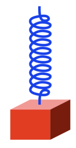
Take a block that’s reasonably heavy and hang it using a spring so that it looks like this:
Figure 1.
The spring is a little stretched because the weight of the block (which is the result of its mass and the Earth’s gravity) is pulling downwards. (We’ll ignore the fact that the spring is also holding up its own weight. Let’s keep this simple…) However, it doesn’t fall to the floor because the spring is pulling upwards.
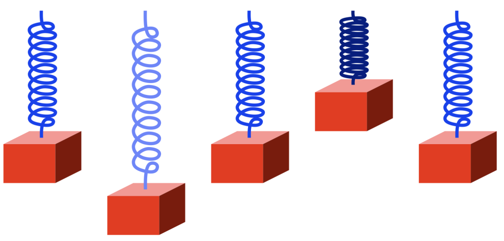
Now pull downwards on the block, so it will look like the example on the right in the figure below.
Figure 2.
The spring is stretched because we’re pulling down on the block. The spring is also pulling upwards more, since it’s pulling against the weight of the block PLUS the force that you’re adding in a downwards direction.
Now you let go of the block. What happens?
The spring is pulling “too hard” on the block, so the block starts rising back to where it started (we’ll call that the “resting position”). However, when it gets there, it has inertia (a body in motion tends to stay in motion… until it hits something big…) so it doesn’t stop. As a result, it moves upwards, higher than the resting position. This squeezes the spring until it gets to some point, at which time the block stops, and then starts going back downwards. When it returns to the resting position, it still has inertia, so it passes that point and goes too far down again. I’ve shown this as a series of positions from left to right in the figure below.
Figure 3
If there were no friction, no air around the block, and no friction within the metal molecules of the spring, then this would bounce up and down forever.
However, there is friction, so some of the movement (“kinetic energy”) is turned into heat and lost. So, each bounce gets smaller and smaller and the maximum velocity of the block (as it passes the resting position) gets lower and lower, until, eventually, it stops moving (at the resting position, where it started).
Notice that I changed the colour of the spring to show when it’s more stretched (lighter blue) and when it’s more compressed (darker blue).
If everything were behaving perfectly, then the RATE at which the bounce repeats wouldn’t change. Only its amplitude (or the excursion of the block, or the height of the bounce) would reduce over time. That bounce rate (let’s say 1 bounce per second, and by “bounce” I mean a full cycle of moment down, up, and back down to where it started again) is the frequency of the repetition (or oscillation).
If you make the weight lighter, then it will bounce faster (because the spring can pull the weight more “easily”). If you make the spring stiffer, then it will bounce faster (because the spring can pull the weight more “easily”). So, we can change the frequency of the oscillation by changing the weight of the block or the stiffness of the spring.
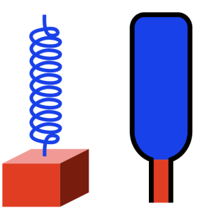
Now take a look at the same weight on a spring next to an up-side down wine bottle that (sadly) has been emptied of wine.
Figure 4.
Notice that I’ve added some colours to the air inside the bottle. The air in the bottle itself is blue, just like the colour of the spring. This is because, if we pull air out of the bottle (downwards), the air inside it will pull back (upwards; just like the metal spring pulling back upwards on the block). I’ve made the small cylinder of air in the neck of the bottle red, just like the block. This is because that air has some mass, and it’s free to move upwards (into the bottle) and downwards (out of the bottle) just like the block.
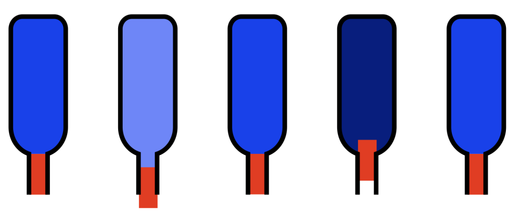
If I were somehow able to pull the “plug” of air out of the neck of the bottle, the air inside would try to pull it back in. If I then “let go”, the plug would move inwards, go too far (because it also has inertia), squeezing (or compressing) the air inside the bottle, which would then push the plug back out. This is shown in the figure below.
Figure 5.
At the level we’re dealing with, this behaviour is practically identical to the behaviour of the block on the spring. In other words, although the block and the plug are made of different materials, and although the metal spring and the air inside the bottle are different materials, Figures 3 and 5 show the same behaviour of the same kind of system.
How do you pull the plug of air out of the bottle? It’s probably easier to start by pushing it inwards instead, by blowing across the top.
When you do this, a little air leaks into the opening, pushing the plug inwards. The “spring” in the bottle then pushes the plug outwards, and your cycle has started. If you wanted to do the same thing with the block, you’d lift it and let go to start the oscillation.
However, you don’t need to blow across the bottle to make it oscillate. You can just tap it with the palm of your hand, for example. Or, if you put the bottle next to your ear and listen carefully, you’ll hear a note “singing along” with the sound in the room. This is because the air in the bottle resonates; it moves back and forth very easily at the frequency that’s determined by the mass of the air in the neck and the volume of air in of the bottle (the spring).
However, remember that friction can make the oscillation decay (or die away) faster, by turning the movement into heat.
One last thing…
There’s another way to get either the block or the wine bottle oscillating:
You can move the TOP of the spring (for example, if you pull it up, then the spring will pull the block upwards, and it’ll start bouncing). Or, you could tap the bottom of the wine bottle (which is on the top in my drawings).
This method of starting the oscillation will come in handy in part 2.
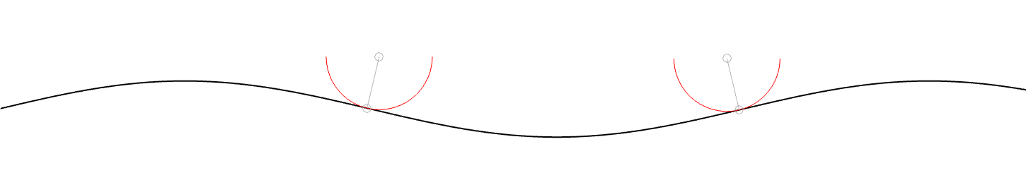
In the last posting, I showed a scale drawing of a 15 µm radius needle on a 1 kHz sine tone with a modulation velocity of 50 mm/s (peak) on the inside groove of a record. Looking at this, we could see that the maximum angular rotation of the contact point was about 13º away from vertical, so the total range of angular rotation of that point would be about 27º.
I also mentioned that, because vinyl is mastered so that the signal on the groove wall has a constant velocity from about 1 kHz and upwards, then that range will not change for that frequency band. Below 1 kHz, because the mastering is typically ensuring a constant amplitude on the groove wall, then the range decreases with frequency.
We can do the math to find out exactly what the angular rotation the contact point is for a given modulation velocity and groove speed.
Figure 1: A scale drawing of a 15 µm radius needle on a 1 kHz sine tone with a modulation velocity of 50 mm/s (peak) on the inside groove of a record. These two points are the two extremes of the angular rotation of the contact point.
Looking at Figure 1, the rotation is ±13.4º away from vertical on the maximum; so the total range is 26.8º. We convert this to a time modulation by converting that angular range to a distance, and dividing by the groove speed at the location of the needle on the record.
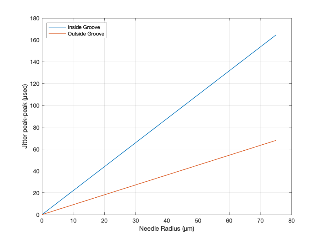
If we repeat that procedure for a range of needle radii from 0 µm to 75 µm for the best-case (the outside groove) and the worst-case (the inside groove), we get the results shown in Figure 2.
Figure 2. The peak-to-peak equivalent “jitter” values of the inside and outside grooves for a range of needle radii.
Back in Part II of what is turning out to be a series of postings on this topic, I wrote
If this were a digital system instead of an analogue one, we would be describing this as ‘signal-dependent jitter’, since it is a time modulation that is dependent on the slope of the signal. So, when someone complains about jitter as being one of the problems with digital audio, you can remind them that vinyl also suffers from the same basic problem…
As I was walking the dog on another night, I got to thinking whether it would be possible to compare this time distortion to the jitter specifications of a digital audio device. In other words, is it possible to use the same numbers to express both time distortions? That question led me here…
Remember that the effect we’re talking about is caused by the fact that the point of contact between the playback needle and the surface of the vinyl is moving, depending on the radius of the needle’s curvature and the slope of the groove wall modulation. Unless you buy a contact line needle, then you’ll see that the radius of its curvature is specified in µm – typically something between about 5 µm and 15 µm, depending on the pickup.
Now let’s do some math. The information and equations for these calculations can be found here.
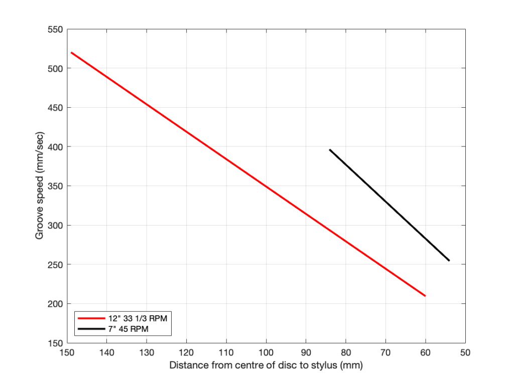
We’ll start with a record that is spinning at 33 1/3 RPM. This means that it makes 0.556 revolutions per second.
The Groove Speed relative to the needle is dependent on the rotation speed and the radius – the distance from the centre of the record to the position of the needle. On a 12″ LP, the groove speed at the outside groove where the record starts is 509.8 mm/sec. At the inside groove at the end of the record, it’s 210.6 mm/sec.
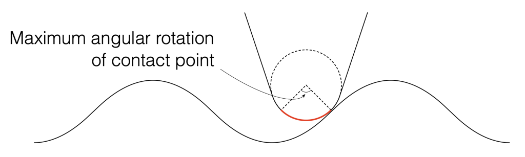
Let’s assume that the angular rotation of the contact point (shown in Figure 1) is 90º. This is not based on any sense of scale – I just picked a nice number.
Figure 1. Artists rendition of the range of the point of contact between the surface of the vinyl and the pickup needle.
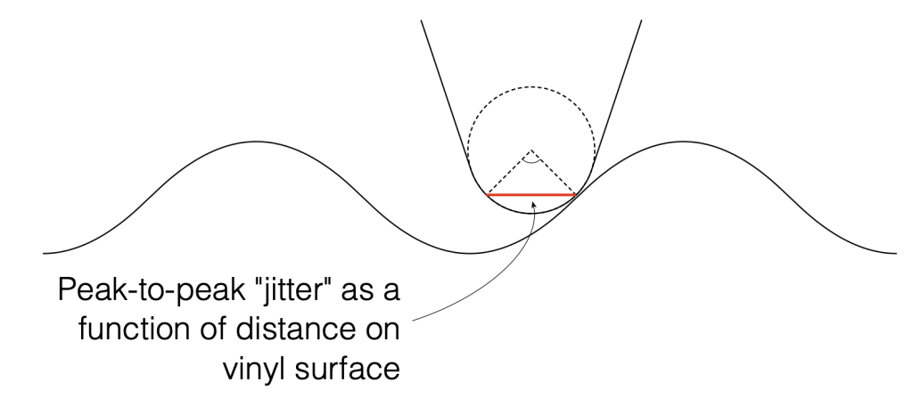
We can convert that angular shift into a shift in distance on the surface of the vinyl by finding the distance between the two points on the surface, as shown below in Figure 2. Since you might want to choose an angular rotation that is not 90º, you can do this with the following equation:
2 * sin(AngularRotation / 2) * radius
So, for example, for a needle with a radius of 10 µm and a total angular rotation of 90º, the distance will be:
2 * sin(90/2) * 10 = 14.1 µm
Figure 2. The angular range from Figure 1 converted to a linear distance on the vinyl’s surface.
We can then convert the “jitter” as a distance to a jitter in time by dividing it by the distance travelled by the needle each second – the groove speed in µm per second. Since that groove speed is dependent on where the needle is on the record, we’ll calculate it as best-case and a worst-case values: at the outside and the inside of the record.
Jitter Distance / Groove Speed = Jitter in time
For example, at the inside of the record where the jitter is worst (because the wavelength is shortest and therefore the maximum slope is highest), the groove speed is about 210.6 mm/sec or 210600 µm/sec.
Then the question is “what kind of jitter distance should we really expect?”
Figure 3. Scale drawing of a needle on a record.
Looking at Figure 3 which shows a scale drawing of a 15 µm radius needle on a 1 kHz tone with a modulation velocity of 50 mm/s (peak) on the inside groove of a record, we can see that the angular rotation at the highest (negative) slope is about 13.4º. This makes the total range about 27º, and therefore the jitter distance is about 7.0 µm.
If we have a 27º angular rotation on a 15 µm radius needle, then the jitter will be
7.0 / 210600 = 0.0000332 or 33.2 µsec peak-to-peak
Of course, as the radius of the needle decreases, the angular rotation also decreases, and therefore the amount of “jitter” drops. When the radius = 0, then the jitter = 0.
It’s also important to note that the jitter will be less at the outside groove of the record, since the wavelength is longer, and therefore the slope of the groove is lower, which also reduces the angular rotation of the contact point.
Since the groove on records are typically equalised to ensure that you have a (roughly) constant velocity above 1 kHz and a constant amplitude below, then this means that the maximum slope of the signal and therefore the range of angular rotation of the contact point will be (roughly) the same from 1 kHz to 20 kHz. As the frequency of the signal descended from 1 kHz and downwards, the amplitude remains (roughly) the same, so the velocity decreases, and therefore the range of the angular rotation of the contact point does as well.
In other words, the amount of jitter is 0 at 0 Hz, and increases with frequency until about 1 kHz, then it remains the same up to 20 kHz.
As one final thing: as I was drawing Figure 3, I also did a scale drawing of a 20 kHz signal with the same 50 mm/s modulation velocity and the same 15 µm radius needle. It’s shown in Figure 4.
Figure 4. Scale drawing of a needle on a record.
As you can see there, the needle’s 15 µm radius means that it can’t drop into the trough of the signal. So, that needle is far too big to play a CD-4 quad record (which can go all the way up to 45 kHz).
After writing the previous posting, I couldn’t stop thinking about it. Mostly, I wanted to get a better idea of the shape of the waveform that results from the difference in a groove cut with a stylus and a spherically-tipped needle on a turntable pickup. To be perfectly honest, I’m not even interested in a ‘real’ simulation. I just wanted to get an intuitive idea of what’s happening down at that nearly-microscopic level. So, I used Matlab to draw some pictures.
Let’s take one period of a sine wave cut into the vinyl master with a chisel-shaped stylus:
Figure 1: The black line shows the wave cut into the vinyl surface. The grey shapes are “artist’s renditions” of the chisel-shaped stylus that cut it.
In theory, the pickup needle tracks this vertical movement exactly, as shown in Figure 2.
Figure 2. The black line is the original signal. The Red line is the signal tracked by a needle that has the same shape as the cutting stylus.
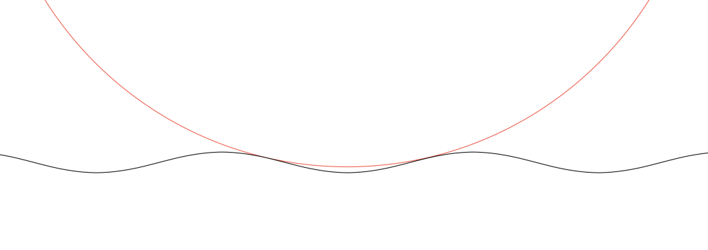
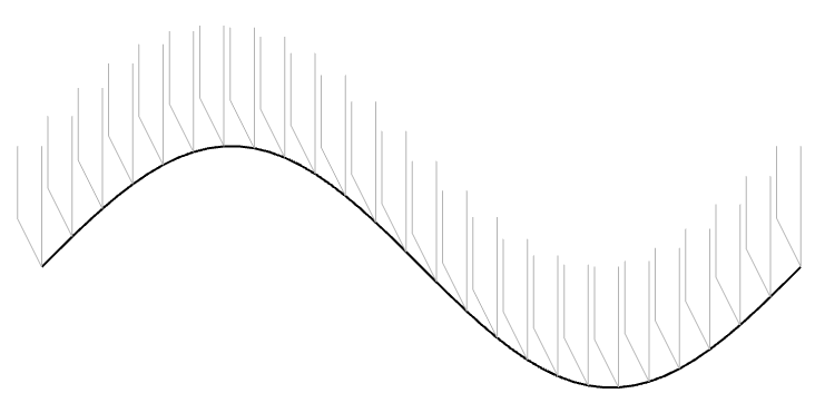
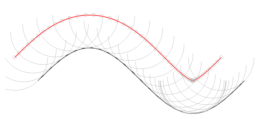
However, we already know that the pickup needle is NOT the same shape as the cutting stylus. In 1964, the needle would have had a spherical tip, which I’ve shown in Figure 3 as a series of semicircles (certainly NOT to scale…).
Figure 3: The black line is the original signal. The grey semicircles are the outline of a spherically-tipped pickup needle. The small grey circles are the centres of those semicircles. When you connect those circles, you get the red line.
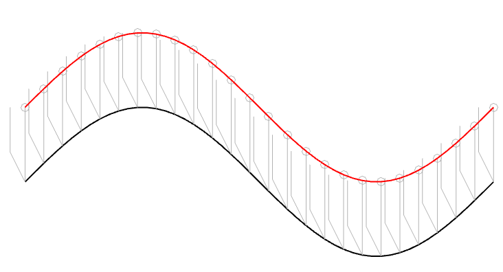
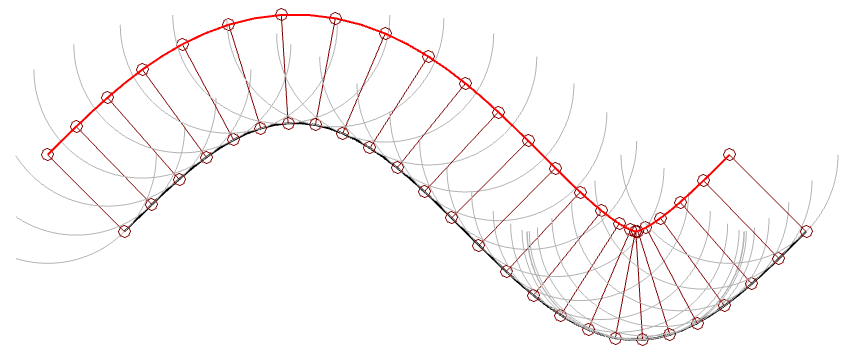
In Figure 3, I’ve connected the centres of the semicircles to make the red line. However, you may notice that this line is not directly above the black line because of the interaction between the slope of the original signal and the radius of the ‘sphere’ that I’m showing. This might be easier to see in Figure 4 which is the same as Figure 3, but I’ve ‘connected the dots’.
Figure 4. This is the same as Figure 3, but I’ve shown the radii of the ‘spheres’ connecting the centre to the surface where it’s touching the vinyl.
(1) One interesting thing about the figure above is that it shows that the point where the needle is resting on the vinyl surface isn’t always vertical – it’s 90º from the tangent of the groove wall (assuming a spherically-ground needle). This means that the output of the needle (which, we assume is determined only by its vertical movement) is actually sliding forwards and backwards in time on the recording, depending on whether the slope is positive or negative.
For example, if you look at the far left of Figure 4, you can see that the centre of the needle is to the left of the point where it’s touching the vinyl. If this is drawn so that the vinyl is moving from right to left (or the needle is moving from left to right – so it’s drawn from the perspective of someone looking in from the edge of the record) then this means that the output of the system is looking ahead in time.
When the needle drops back downwards, it’s delaying the signal, looking back in time.
If this were a digital system instead of an analogue one, we would be describing this as ‘signal-dependent jitter’, since it is a time modulation that is dependent on the slope of the signal. So, when someone complains about jitter as being one of the problems with digital audio, you can remind them that vinyl also suffers from the same basic problem…
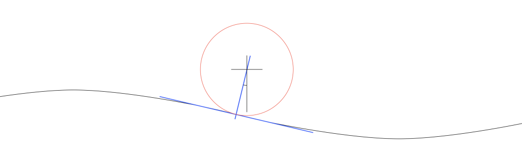
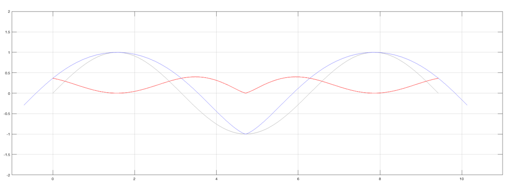
(2) Another interesting thing is that, if we subtract the original signal on the vinyl’s surface from the actual path traced by the needle, we can see the tracing error itself. This is shown below as the red curve in Figure 5.
Figure 5. The original signal is in grey, the movement of the needle is in blue, and the difference (the tracing error) is in red.
Notice that, although the original signal is symmetrical, the blue curve (the actual signal) is not. This means that it has a DC offset, which is easily seen in the error curve in red, which never drops below the vertical 0 line; the mean of the original signal.
(Remember, I’m exaggerating everything here just to get an intuitive understanding of what’s going on.)
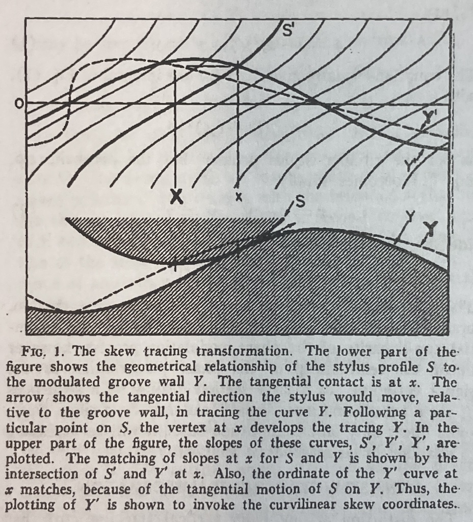
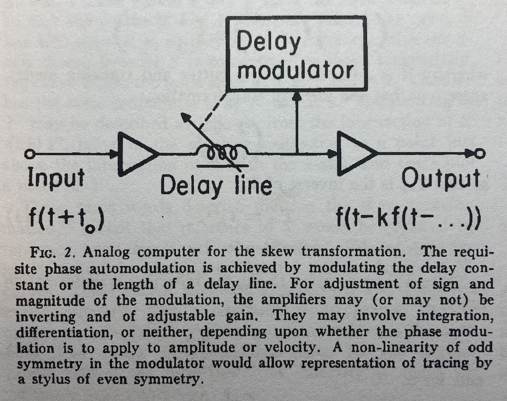
Although I’ve done all of this analysis numerically using Matlab, I’ve also found a paper that describes this error analytically. It’s “Integrated Treatment of Tracing and Tracking Error” by Duane H. Cooper in the Journal of the Audio Engineering Society from January, 1964. In that paper, he shows the following drawing shown below in Figure 6. Compare the dotted line to the blue one above, for example. (It seems that I wasted my time doing math when I should have been reading old papers instead…)
Figure 6.
The horizontal distance in Figure 6 between the bold capital ‘X’ and the small ‘x’ is an angular rotation from the centre of the needle’s spherical tip and therefore a time shift in the playback of the recording. Later in the same paper, Cooper proposes an analogue computer that can predict this distortion by modulating a delay applied to the audio signal as a function of the signal itself. A representation of this from the paper is shown below in Figure 7. This prediction can then be used to generate the pre-emphasis distortion of RCA’s “Dynamic Styli Correlator”.
Figure 7.
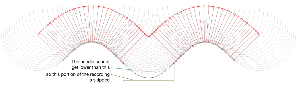
(3) The last thing that I’ve found is an extreme case that should never happen in real life, but it might. This is when the trough that the needle is dropping into is narrower than the diameter of the stylus. When this happens, the point where the stylus is touching jumps instantaneously from one side of the trough to the other. This is shown in Figure 8.
Figure 8. When the stylus is too big to fit into the trough, parts of the waveform are skipped.
This is the same thing that happens when a tire of your car drops into a bad pothole. You roll off one edge of the hole, and hit the edge on the opposite side, but the part of the tire that is actually IN the pothole never actually touches the bottom.
This problem is the same as I described above; but instead of the output signal merely sliding in time, it’s jumping. One example I can think where this would happen in real life is when you play a CD-4 quad LP with a needle that isn’t made for it. However, in this case you won’t notice the problem, since the high-frequency FM modulated surround channels result in a more-or-less constant “ripple” on the groove wall. This means that your needle is just surfing along the tops of the ripples and never drops into a trough at all.
Many audio recording systems are based on a concept known as “pre-emphasis” and “de-emphasis”. This is a process where a signal is distorted (here, I use the word “distorted” to mean “changed”, not “clipped”) at the recording or encoding process to counter-act the effects of something that will happen at playback. One example of this is a RIAA equalisation that applies an overall bass-heavy tilt to the frequency response at playback, and therefore the signal is given the opposite tilt when it’s cut onto the vinyl master. Dolby noise reduction for analogue magnetic tape follows a similar philosophy.
Another type of intentional distortion applied to an audio signal is based on assumptions of what happens at playback. Mixing engineers for television often emphasise lower frequency bands, assuming that everyone’s television loudspeakers needed some help. Pop and rock recording engineers check the mix on a low-quality mono loudspeaker and may make adjustments to the mix – to make sure it survived a clock radio or a portable Bluetooth loudspeaker (depending on which decade we’re talking about). Stereo vinyl records can’t have big low-frequency differences in the two audio channels otherwise the needle will hop out of the groove, so they’re mixed and mastered accordingly.
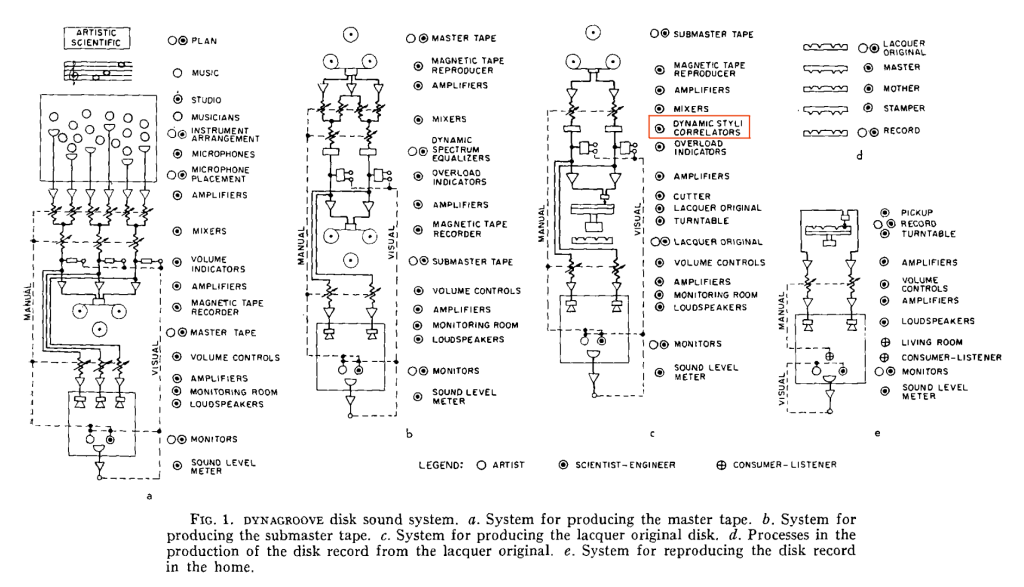
I’ve been reading “The RCA Victor Dynagroove System”, by Harry F. Olsen, published in the April 1964 issue of the Journal of the Audio Engineering Society. In it, he describes the entire recoding chain, including something that piqued my interest called a “Dynamic Styli Correlator” which is a distortion that is applied to the audio at almost the last stage of the signal path before it reaches the cutter head of the lathe that creates the lacquer master. You can see it here in Figure 1 from the article (I drew the red box around it).
Cool name; almost worthy of Dr. Heinz Doofenshmirtz (although it’s missing the “-inator”). But what is it?
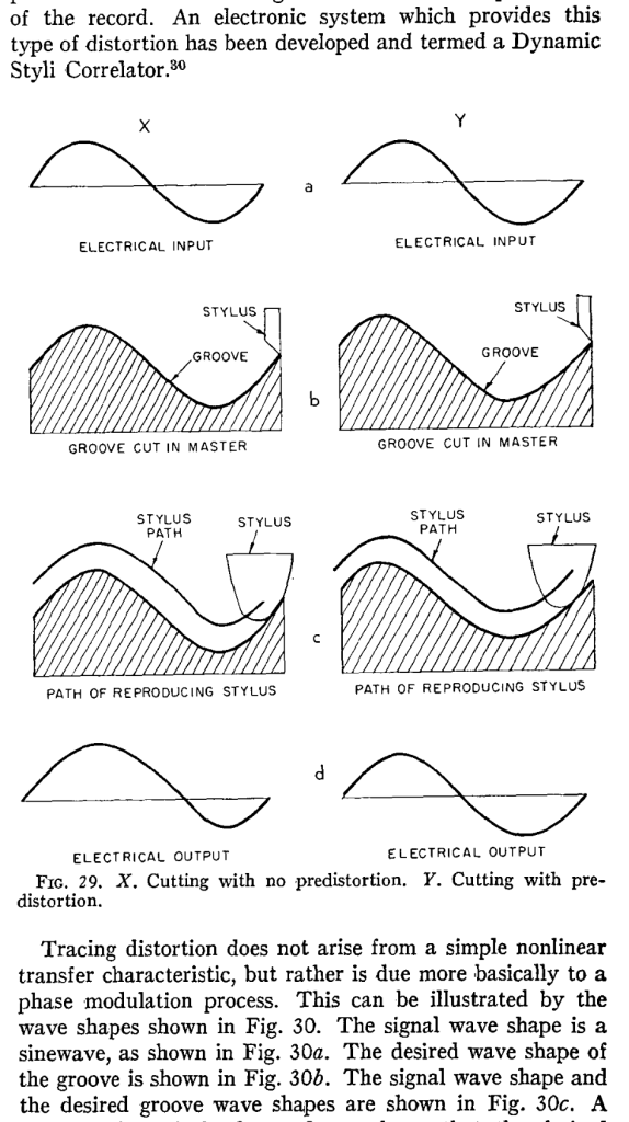
One of the problems with playing back a vinyl record is that the shape of the needle on your turntable is not the same shape as the cutting stylus on the lathe. Consequently, the path that the needle tracks is not exactly the same as the path of the stylus. The result of this mis-match is that the electrical input signal that is used to make the master (the original recording) is not the same as the electrical output signal that comes out of your turntable (what you hear).
The idea behind the Dynamic Styli Correlator was that the actual path of the playback needle could be predicted, and the groove cut by the stylus could be modified to ensure that the output was correct. In other words, the distortion caused by the playback needle was estimated, and a distorted groove was cut to make the needle behave. This is shown graphically in Figure 29 of the article:
This is a great idea if the system works and if the prediction of the playback needle’s path is correctly predicted. However, neither of these two assumptions is guaranteed; so a number of things can go wrong here, and if anything can go wrong, it probably will.
However, it does mean at least as a start, that if you play an old RCA Victor Dynagroove record with a stylus shape that wasn’t invented yet in 1964 (say, a contact line stylus made for CD-4 Quadraphonic records, for example). Then you might wind up doing a much better job of reproducing the distortion that RCA created in the first place, instead of what they thought you were supposed to hear.
Back when I was at McGill, one of my fellow Ph.D. students was Mark Ballora, who did his doctorate in converting heart rate data to an audible signal that helped doctors to easily diagnose patients suffering from sleep apnea.
When you look at the datasheet of an audio device, you may see a specification that states its “signal to noise ratio” or “SNR”. Or, you may see the “dynamic range” or “DNR” (or “DR”) lists as well, or instead.
These days, even in the world of “professional audio” (whatever that means), these two things are similar enough to be confused or at least confusing, but that’s because modern audio devices don’t behave like their ancestors. So, if we look back 30 years ago and earlier, then these two terms were obviously different, and therefore independently usable. So, in order to sort this out, let’s take a look at the difference in old audio gear and the new stuff.
Let’s start with two of basic concepts:
All audio devices (or storage media or transmission systems) make noise. If you hold a resistor up in the air and look at the electrical difference across its two terminals and you’ll see noise. There’s no way around this. So, an amplifier, a DAC, magnetic tape, a digital recording stored on a hard drive… everything has some noise floor at the bottom that’s there all the time.
All audio devices have some maximum limit that cannot be exceeded. A woofer can move in and out until it goes so far that it “bottoms out” on the magnet or rips the surround. A power amplifier can deliver some amount of current, but no higher. The headphone output on your iPhone cannot exceed some voltage level.
So, the goal of any recording or device that plays a recording is to try and make sure that the audio signal is loud enough relative to that noise that you don’t notice it, but not so loud that the limit is hit.
Now we have to look a little more closely at the details of this…
If we take the example of a piece of modern audio equipment (which probably means that it’s made of transistors doing the work in the analogue domain, and there’s lots of stuff going on in the digital domain) then you have a device that has some level of constant noise (called the “noise floor”) and maximum limit that is at a very specific level. If the level of your audio signal is just a weeee bit (say, 0.1 dB) lower than this limit, then everything is as it should be. But once you hit that limit, you hit it hard – like a brick wall. If you throw your fist at a brick wall and stop your hand 1 mm before hitting it, then you don’t hit it at all. If you don’t stop your hand, the wall will stop it for you.
In older gear, this “brick wall” didn’t exist in lots of gear. Let’s take the sample of analogue magnetic tape. It also has a noise floor, but the maximum limit is “softer”. As the signal gets louder and louder, it starts to reach a point where the top and bottom of the audio waveform get increasingly “squished” or “compressed” instead of chopping off the top and bottom.
I made a 997 Hz sine wave that starts at a very, very low level and increases to a very high level over a period of 10 seconds. Then, I put it through two simulated devices.
Device “A” is a simulation of a modern device (say, an analogue-to-digital converter). It clips the top and bottom of the signal when some level is exceeded.
Device “B” is a simulation of something like the signal that would be recorded to analogue magnetic tape and then played back. Notice that it slowly “eases in” to a clipped signal; but also notice that this starts happening before Device “A” hits its maximum. So, the signal is being changed before it “has to”.
Let’s zoom in on those two plots at two different times in the ramp in level.
Device “A” is the two plots on the top at around 8.2 seconds and about 9.5 seconds from the previous figure. Device “B” is the bottom two plots, zooming in on the same two moments in time (and therefore input levels).
Notice that when the signal is low enough, both devices have (roughly) the same behaviour. They both output a sine wave. However, when the signal is higher, one device just chops off the top and bottom of the sine wave whereas the other device merely changes its shape.
Now let’s think of this in terms of the signals’ levels in relationship to the levels of the noise floors of the devices and the distortion artefacts that are generated by the change in the signals when they get too loud.
If we measure the output level of a device when the signal level is very, very low, all we’ll see is the level of the inherent noise floor of the device itself. Then, as the signal level increases, it comes up above the noise floor, and the output level is the same as the level of the signal. Then, as the signal’s level gets too high, it will start to distort and we’ll see an increase in the level of the distortion artefacts.
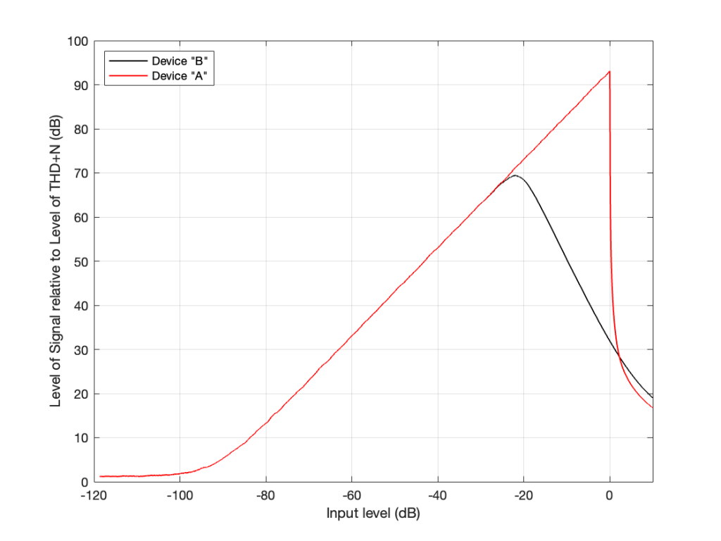
If we plot this as a ratio of the signal’s level (which is increasing over time) to the combined level of the distortion and noise artefacts for the two devices, it will look like this:
On the left side of this plot, the two lines (the black door Device “A” and the red for Device “B”) are horizontal. This is because we’re just seeing the noise floor of the devices. No matter how much lower in level the signals were, the output level would always be the same. (If this were a real, correct Signal-to-THD+N ratio, then it would actually show negative values, because the signal would be quieter than the noise. It would really only be 0 dB when the level of the noise was the same as the signal’s level.)
Then, moving to the right, the levels of the signals come above the noise floor, and we see the two lines increasing in level.
Then, just under a signal level of about -20 dB, we see that the level of the signal relative to the artefacts starts in Device “B” reaches a peak, and then starts heading downwards. This is because as the signal level gets higher and higher, the distortion artefacts increase in level even more.
However, Device “A” keeps increasing until it hits a level 0 dB, at which point a very small increase in level causes a very big jump in the amount of distortion, so the relative level of the signal drops dramatically (not because the signal gets quieter, but because the distortion artefacts get so loud so quickly).
Now let’s think about how best to use those two devices.
For Device “A” (in red) we want to keep the signal as loud as possible without distorting. So, we try to make sure that we stay as close to that 0 dB level on the X-axis as we can most of the time. (Remember that I’m talking about a technical quality of audio – not necessarily something that sounds good if you’re listening to music.) HOWEVER: we must make sure that we NEVER exceed that level.
However, for Device “B”, we want to keep the signal as close to that peak around -20 dB as much as possible – but if we go over that level, it’s no big deal. We can get away with levels above that – it’s just that the higher we go, the worse it might sound because the distortion is increasing.
Notice that the red line and the black line cross each other just above the 0 dB line on the X-axis. This is where the two devices will have the same level of distortion – but the distortion characteristics will be different, so they won’t necessarily sound the same. But let’s pretend that the the only measure of quality is that Y-axis – so they’re the same at about +2 dB on the X-axis.
Now the question is “What are the dynamic ranges of the two systems?” Another way to ask this question is “How much louder is the loudest signal relative to the quietest possible signal for the two devices?” The answer to this is “a little over 100 dB” for both of them, since the two lines have the same behaviour for low signals and they cross each other when the signal is about 100 dB above this (looking at the X-axis, this is the distance between where the two lines are horizontal on the left, and where they cross each other on the right). Of course, I’m over-simplifying, but for the purposes of this discussion, it’s good enough.
The second question is “What are the signal-to-noise ratios of the two systems?” Another way to ask THIS question is “How much louder is the average signal relative to the quietest possible signal for the two devices?” The answer to this question is two different numbers.
Device “A” has a signal-to-noise ratio of about 100 dB , because we’re going to use that device, trying to keep the signal as close to clipping as possible without hitting that brick wall. In other words, for Device “A”, the dynamic range and the signal-to-noise ratio are the same because of the way we use it.
Device “B” has a signal-to-noise ratio of about 80 dB because we’re going to try to keep the signal level around that peak on the black curve (around -20 dB on the X-axis). So, its signal-to-noise ratio is about 20 dB lower than its dynamic range, again, because of the way we use it.
The problem is, these days, a lot of engineers aren’t old enough to remember the days when things behaved like Device “B”, so they interchange Signal to Noise and Dynamic Range all willy-nilly. Given the way we use audio devices today, that’s okay, except when it isn’t.
For example, if you’re trying to connect a turntable (which plays vinyl records that are mastered to behave more like Device “B”) to a digital audio system, then the makers of those two systems and the recordings you play might not agree on how loud things should be. However, in theory, that’s the problem of the manufacturers, not the customers. In reality, it becomes the problem of the customers when they switch from playing a record to playing a digital audio stream, since these two worlds treat levels differently, and there’s no right answer to the problem. As a result, you might need to adjust your volume when you switch sources.
Last week, I was doing a lecture about the basics of audio and I happened to mention one of the rules of thumb that we use in loudspeaker development:
If you have a single loudspeaker driver and you want to keep the same Sound Pressure Level (or output level) as you change the frequency, then if you go down one octave, you need to increase the excursion of the driver 4 times.
One of the people attending the presentation asked “why?” which is a really good question, and as I was answering it, I realised that it could be that many people don’t know this.
Let’s take this step-by-step and keep things simple. We’ll assume for this posting that a loudspeaker driver is a circular piston that moves in and out of a sealed cabinet. It is perfectly flat, and we’ll pretend that it really acts like a piston (so there’s no rubber or foam surround that’s stretching back and forth to make us argue about changes in the diameter of the circle). Also, we’ll assume that the face of the loudspeaker cabinet is infinite to get rid of diffraction. Finally, we’ll say that the space in front of the driver is infinite and has no reflective surfaces in it, so the waveform just radiates from the front of the driver outwards forever. Simple!
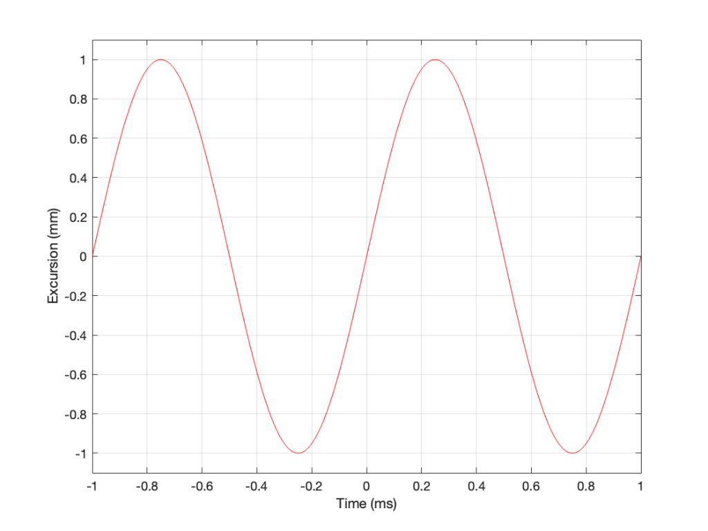
Then, we’ll push and pull the loudspeaker driver in and out using electrical current from a power amplifier that is connected to a sine wave generator. So, the driver moves in and out of the “box” with a sinusoidal motion. This can be graphed like this:
Figure 1: The excursion of a loudspeaker driver playing a 1 kHz sine wave at some output level.
As you can see there, we have one cycle per millisecond, therefore 1000 cycles per second (or 1 kHz), and the driver has a peak excursion of 1 mm. It moves to a maximum of 1 mm out of the box, and 1 mm into the box.
Consider the wave at Time = 0. The driver is passing the 0 mm line, going as fast as it can moving outwards until it gets to 1 mm (at Time = 0.25 ms) by which time it has slowed down and stopped, and then starts moving back in towards the box.
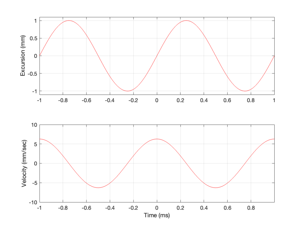
So, the velocity of the driver is the slope of the line in Figure 1, as shown in Figure 2.
Figure 2: The excursion and velocity of the same loudspeaker driver playing the same signal.
As the loudspeaker driver moves in and out of the box, it’s pushing and pulling the air molecules in front of it. Since we’ve over-simplified our system, we can think of the air molecules that are getting pushed and pulled as the cylinder of air that is outlined by the face of the moving piston. In other words, its a “can” of air with the same diameter as the loudspeaker driver, and the same height as the peak-to-peak excursion of the driver (in this case, 2 mm, since it moves 1 mm inwards and 1 mm outwards).
However, sound pressure (which is how loud sounds are) is a measurement of how much the air molecules are compressed and decompressed by the movement of the driver. This is proportional to the acceleration of the driver (neither the velocity nor the excursion, directly…). Luckily, however, we can calculate the driver’s acceleration from the velocity curve. If you look at the bottom plot in Figure 2, you can see that, leading up to Time = 0, the velocity has increased to a maximum (so the acceleration was positive). At Time = 0, the velocity is starting to drop (because the excursion is on its was up to where it will stop at maximum excursion at time = 0.25 ms).
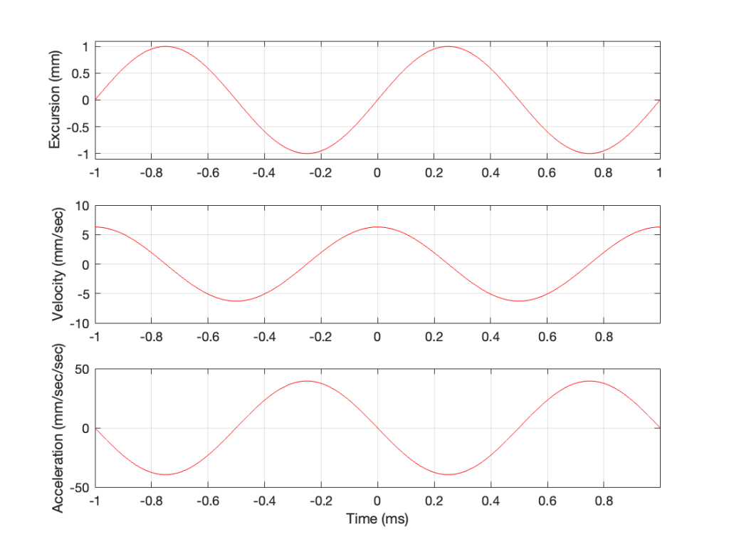
In other words, the acceleration is the slope of the velocity curve, the line in the bottom plot in Figure 2. If we plot this, it looks like Figure 3.
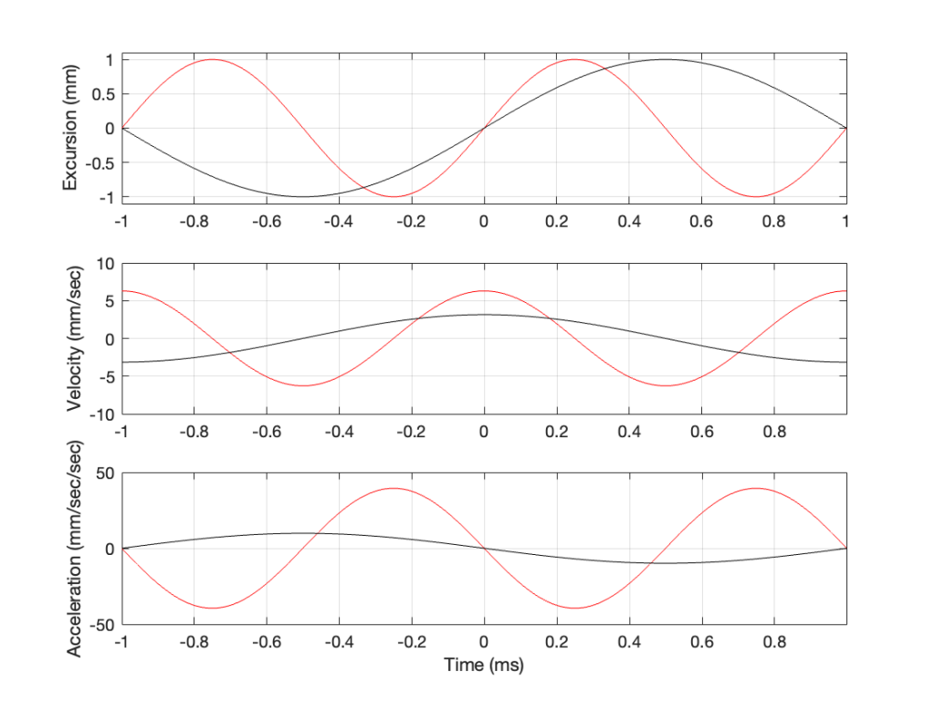
Figure 3: The excursion, velocity and acceleration of the same loudspeaker driver playing the same signal.
Now we have something useful. Since the bottom plot in Figure 3 shows us the acceleration of the driver, then it can be used to compare to a different frequency. For example, if we get the same driver to play a signal that has half of the frequency, and the same excursion, what happens?
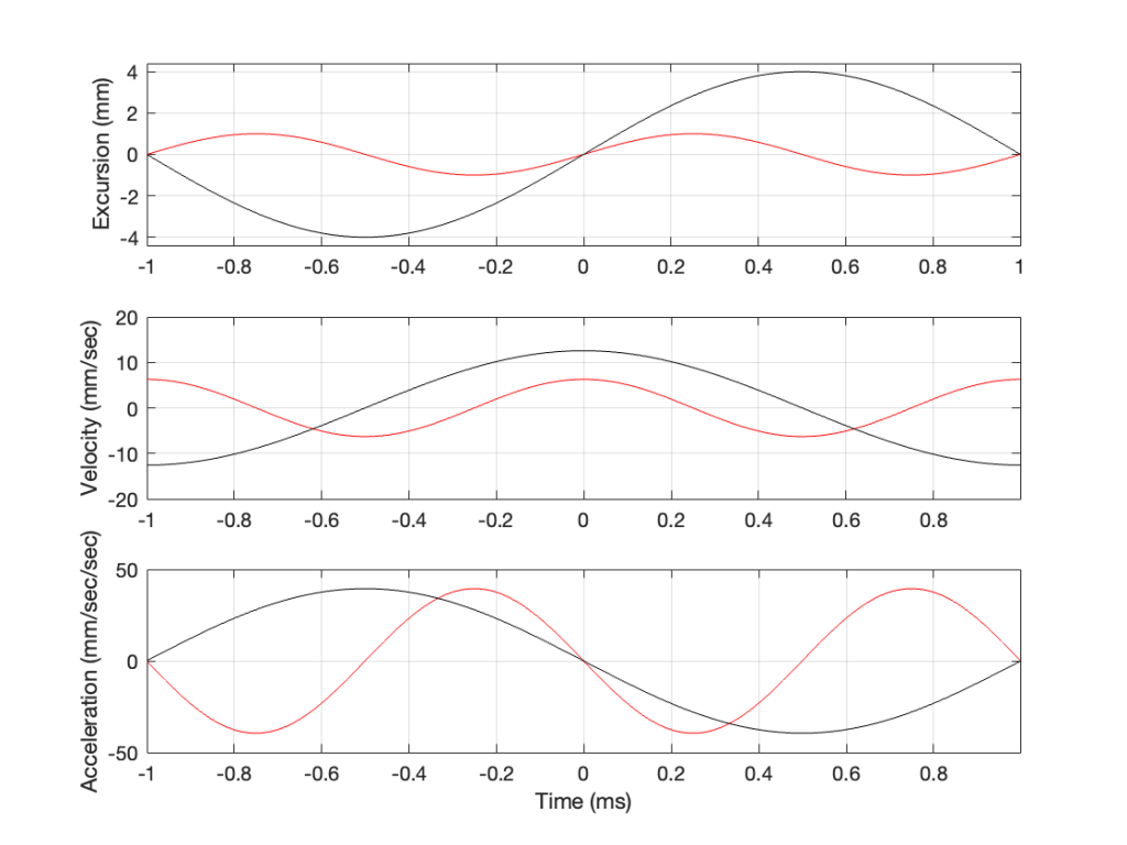
Figure 4: Comparing the excursion, velocity and acceleration of the same loudspeaker driver playing two different signals with the same excursion. (The red line is the same in Figure 4 as in Figure 3.)
In Figure 4, two sine waves are shown: the black line is 1/2 of the frequency of the red line, but they both have the same excursion. If you take a look at where both lines cross the Time = 0 point, then you can see that the slopes are different: the red line is steeper than the black. This is why the peak of the red line in the velocity curve is higher, since this is the same thing. Since the maximum slope of the red line in the middle plot is higher than the maximum slope of the black line, then its acceleration must be higher, which is what we see in the bottom plot.
Since the sound pressure level is proportional to the acceleration of the driver, then we can see in the top and bottom plots in Figure 4 that, if we halve the frequency (go down one octave) but maintain the same excursion, then the acceleration drops to 25% of the previous amount, and therefore, so does the sound pressure level (20*log10(0.25) = -12 dB, which is another way to express the drop in level…)
This raises the question: “how much do we have to increase the excursion to maintain the acceleration (and therefore the sound pressure level)?” The answer is in the “25%” in the previous paragraph. Since maintaining the same excursion and multiplying the frequency by 0.5 resulted in multiplying the acceleration by 0.25, we’ll have to increase the excursion by 4 to maintain the same acceleration.
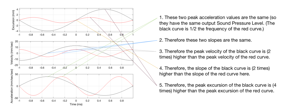
Figure 5: Comparing the excursion, velocity and acceleration of the same loudspeaker driver playing two different signals at two different excursions. Notice that some of the vertical scales in the plots have changed. (The red line is the same in Figure 5 as in Figures 4 and 3.)
Looking at Figure 5: The black line is 1/2 the frequency of the red line. Their accelerations (the bottom plots) have the same peak values (which means that they produce the same sound pressure level). This, means that the slopes of their velocities are the same at their maxima, which, in turn, means that the peak velocity of the black line (the lower frequency) is higher. Since the peak velocity of the black line is higher (by a factor of 2) then the slope of the excursion plot is also twice as steep, which means that the peak of the excursion of the black line is 4x that of the red line. All of that is explained again in Figure 6.
Figure 6. A repeat of Figure 5 with some explanations that (hopefully) help.
Therefore, assuming that we’re using the same loudspeaker driver, we have to increase the excursion by a factor of 4 when we drop the frequency by a factor of 2, in order to maintain a constant sound pressure level.
However, we can play a little trick… what we’re really doing here is increasing the volume of our “cylinder” of air by a factor of 4. Since we don’t change the size of the driver, we have to move it 4 times farther.
However, the volume of a cylinder is
π r2 * height
and we’re just playing with the “height” in that equation. A different way would be to use a different driver with a bigger surface area to play the lower frequency. For example, if we multiply the radius of the driver by 2, and we don’t change the excursion (the “height” of the cylinder) then the total volume increases by a factor of 4 (because the radius is squared in the equation, and 2*2 = 4).
Another way to think of this: if our loudspeaker driver was a square instead of a circle, we could either move it in and out 4 times farther OR we would make the width and the length of the square each twice as big to get the a cube with the same volume. That “r2” in the equation above is basically just the “width * length” of a circle…
This is why woofers are bigger than tweeters. In a hypothetical world, a tweeter can play the same low frequencies as a woofer – but it would have to move REALLY far in and out to do it.
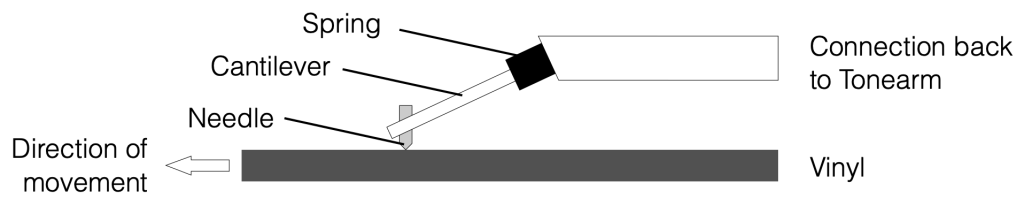
It should not come as a surprise that, when we talk about how a vinyl record works, we can start by looking at the movement of the needle in the groove. If we simplify that connection a little (by reducing the audio signal to one channel, but we’ll come back to that point later), then we can think of this as a needle, sitting on a surface. The needle is at the end of an arm that we call the “cantilever” (because it is fixed on one end and it can move up and down on the other end where the needle is attached) and that cantilever is attached somehow to the tonearm using a springy material of some kind (like rubber, for example).
Figure 1
The simple diagram above shows that arrangement. Of course, I’ve left out a bunch of things, and nothing is to scale, but those details are not important right now.
I’ll make the “spring” in this diagram out of flexible rubber that has some “springiness” or “compliance”. The more compliant the spring, the easier it is to flex. So a stiff spring in not very compliant. (This concept is very important to understand as we go on.)
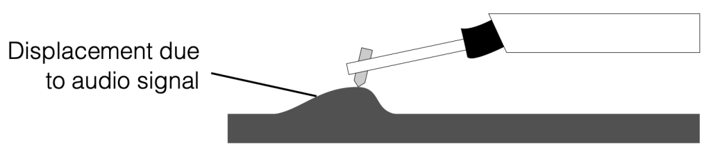
The audio signal is “encoded” into the surface of the vinyl using bumps and dips that cause the needle to move up and down. I’ve shown this in the simple diagram below.
Figure 2
Notice in that diagram that the needle is in contact with the surface of the vinyl, but the part of the system that connects back to the tonearm has not lifted. This is because the connection between the cantilever and the tonearm assembly is compliant enough to let the cantilever move upwards (or downwards) without moving the rest of the system.
Think of this like driving over a very small bump in the road in your car. The compliance of the tires and the shock absorbers will result in the tire riding over the bump, but the car doesn’t jump as a result.
Remember that the bump in the surface of the vinyl is only passing by, so the needle isn’t raised for long. As a result part of the reason the tonearm doesn’t move upwards (and your car doesn’t jump) is partly because it’s heavy. Its mass results in an inertia that “wants” to stop it from moving up and down. (The other factor that’s involved here is an adjustment in the tonearm called the “tracking force” which is a measurement of how much the tonearm is pushing downwards on the needle.)
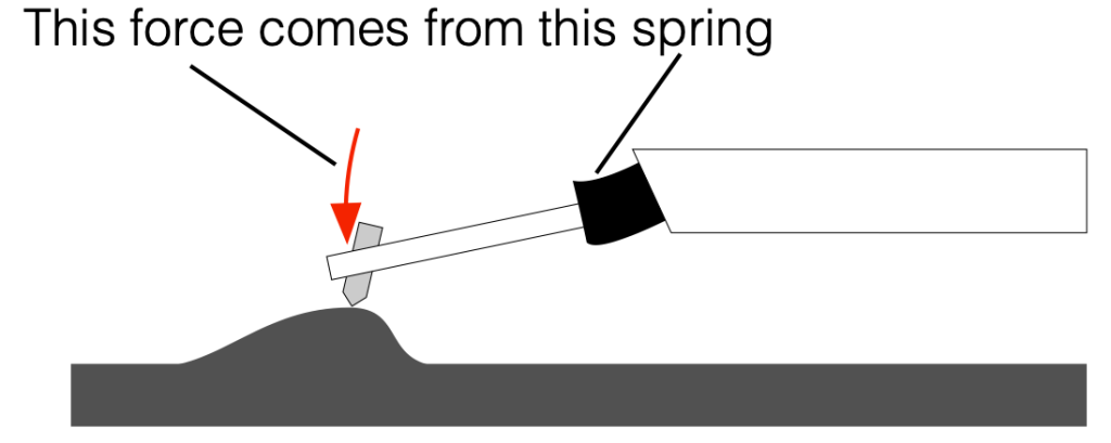
Consequently, when that bump comes along, the needle rides on top of it, and the force that is pushing it downwards comes mostly from the “spring” at the other end of the cantilever, as shown below.
Figure 3
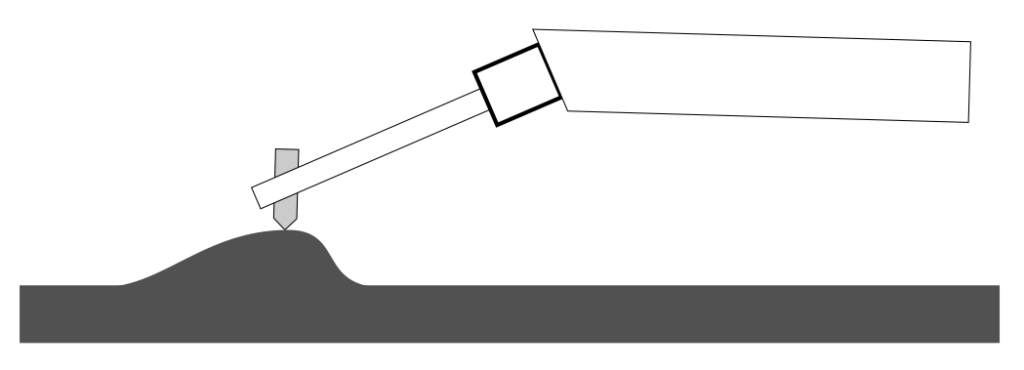
If the spring had no compliance (in other words, if it weren’t a spring, and the cantilever were just connected directly to the tonearm) and if the cantilever and needle were strong enough to take the force, then the entire tonearm assembly would jump up and down instead, as shown below. (Imagine riding in a horse-drawn buggy with wooden wheels with steel rims, and no springs on the axles. You’d feel every single rock on the road…)
Figure 4
The tonearm is resting on two points: one is the tip of the needle and the other is at the other end at the pivot point where it also rotates horizontally as you play the album. If we were really dumb turntable designers, then half of the mass of the tonearm would be resting on the needle (and the other half would be resting on the pivot). This would be bad, since your records would wear out very fast. So, a tonearm has some kind of adjustment on it that reduces the amount of weight on the needle. The simplest way to do this is to put a counterweight on the opposite side of the pivot so it’s more like a see-saw at the playground. As you move the counterweight away from the pickup, the downwards force at the needle gets smaller. In fact, you can probably adjust the counterweight so far that the needle-end of the tonearm is lighter, and it is stuck up in the air…
We adjust the amount of downwards force at the needle (called the “tracking force”) to result in a value that is in balance with the compliance of the connection to the cantilever. If the tracking force is too high (or the compliance is too high for the tracking force) then the tonearm will sink like I’ve shown below.
Figure 5
There are lots of things wrong with this. The first is that the needle isn’t at the correct angle to the surface of the vinyl, so it’s not going to move correctly. The second is that the cantilever is at the wrong angle, so it’s not going to move upwards with the same behaviour as it moves downwards, which results in an asymmetrical distortion of the signal. But possibly the most obvious problem is that there’s just too much downwards pressure on the vinyl, so your records will wear out faster.
So, there is a balance between the tracking force and the compliance. That balance ensures that you always have contact between the tip of the needle and the surface of the vinyl as the bumps and dips go by.
Digging into the details
One of the things I do regularly is to measure the magnitude response of a turntable from the surface of the vinyl to the electrical output of the RIAA preamplifier. In order to do this, I play two tracks on a special test record (Brüel & Kjær QR 2010) which has the following audio signals:
20 Hz to 45 kHz sinusoidal tone, log sweep, 5 sec per decade, Right channel
Sometimes (but very rarely), I notice that the needle will skip (or jump) at the transition between the 1 kHz tone and the start of the sine sweep. If this happens, for track 1, the needle will skip forwards into the sweep.
When this happened the first time I thought “Ah hah! The tracking force isn’t high enough, so the needle is being thrown out of the groove. I just need to adjust it.” But after checking the tracking force with my meter (a very small, very precise and accurate scale), I found out that this was not the problem.
Of course, I could make the problem go away by increasing the tracking force, but then it was too high, and my records (and the needle tip) will wear down faster. This would be covering up the symptom, but not correcting the actual problem.
So, what is the problem? It’s that the compliance of the pickup is too low due to an error in the manufacturing process or the fact that it’s just old and the rubber has stiffened over time. In other words it looks more like the system shown in Figure 4, above.
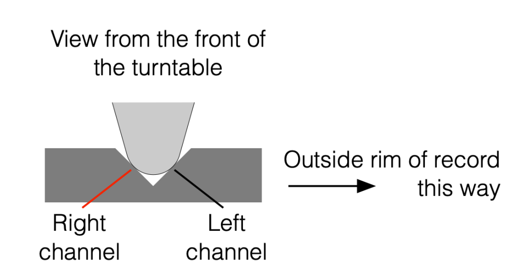
Let’s take a system where the pickup compliance is too low (so the spring is too stiff), so the tonearm can be tossed up off the vinyl surface. We then combine that with the knowledge of how the needle sits in the groove on the vinyl and which channel is on which side of that groove (which I’ve shown below in Figure 6).
Figure 6
Now we can see that, if there’s a bump in the Left channel, it will push the needle on a 45º angle upwards, and if the tracking force and compliance aren’t working together as they should, then the entire tonearm can be pushed hard enough to cause the needle to lift off the surface of the vinyl, heading in towards the centre of the record (towards the left in Figure 6).
What does the signal actually look like?
Let’s go back and look at a recording of that transition between the 1 kHz tone and the start of the 20 Hz sweep, using a pickup that is behaving properly.
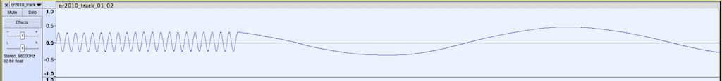
Figure 7
The figure above is a screenshot from Audacity that shows the “raw” signal that I recorded at the input of my sound card which is connected to the output of the RIAA preamplifier. I’ve zoomed in to the moment when the track transitions from the 1 kHz tone to the 20 Hz tone at the start of the sweep.
Let’s now use this to go backwards and try to figure out what the surface of the vinyl looks like. I’ll start by re-creating a “perfect” version of that signal in Matlab by joining a 1 kHz cosine wave to a 20 Hz cosine wave.
Figure 8
You might notice that I’ve changed the value a little. I’m simulating one channel of a tone that has a level of at 5 cm/sec, RMS lateral velocity for two channels, instead of the 3.16 cm/sec from the B&K record. But this doesn’t really matter too much – I’ve just done it to make the numbers look nice and be a little easier to talk about.
I’m simulating a system that has a total gain set so that a modulation velocity of 3.54 cm/sec in one channel will produce 354 mV RMS (500 mV peak) at the output of the RIAA at 1 kHz.
Since the lateral velocity of a two-channel tone is 5 cm/sec, then the velocity of one channel will be 1/sqrt(2) of that value because the groove wall is 45º away from the lateral axis and cos(45º) = 1/sqrt(2).
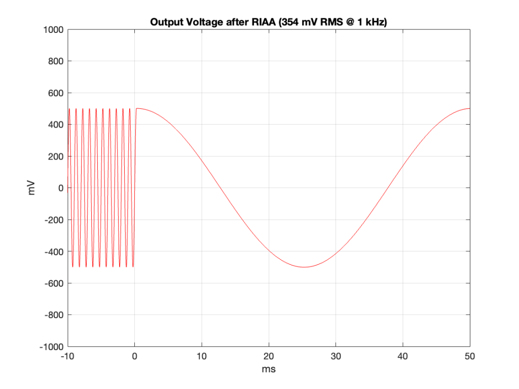
If we take the signal in Figure 8 and filter it with a RIAA pre-emphasis filter (sometime called an “anti-RIAA” or an “inverse RIAA”) and drop the level by 40 dB (a typical gain for a RIAA preamp), then the signal looks like the plot in Figure 9.
Figure 9
As you can see there, the signal much lower in level overall (because of the -40 dB gain) and the 20 Hz tone is much lower in level than the 1 kHz tone (because of the pre-emphasis filter).
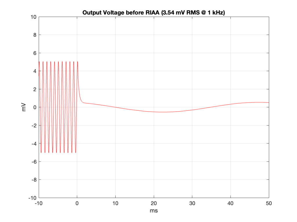
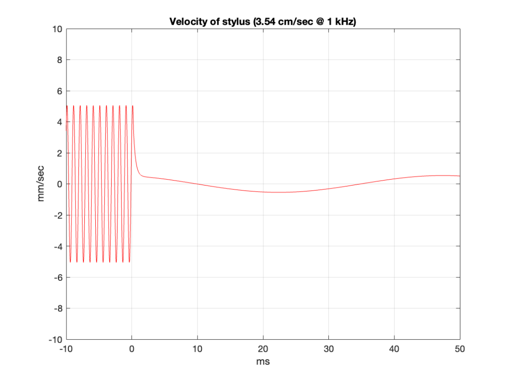
The output of the pickup is a current that is proportional to the velocity of the needle. So, we can move farther backwards in the chain and plot the velocity of the needle over time, shown in Figure 10. As you can see, the shape of this plot looks identical to the one in Figure 9. This is because I’m assuming that the current output of the pickup is in phase with the voltage at the input of the RIAA. (This is a safe assumption for the two frequencies we’re looking at here. If you want to pick a fight with me about this, drop by and do it in person. But you’re buying the beer…)
Figure 10 (I made a mistake in the Y-axis label – it should say cm/sec. I’ll come back and fix that later)
Now comes a jump… the velocity of the needle can be calculated by finding the derivative of the displacement over time, which means that the displacement can be found by integrating the velocity.
If you don’t like calculus, then you can think of it this way: In the old days, if you drove from Struer to Copenhagen, you had to take a ferry to get from the island of Fyn to the island of Zealand. Every once in a while, there would be a policeperson, walking around the parking lot as people waited to board the ferry, handing out speeding tickets to some of the people there. What happened was that the licence plates were recorded with time stamps as they crossed the bridge to Fyn from Jutland – which is about 75 km away from the parking lot. If you arrive at the ferry too early, you must have been speeding, and you get rewarded with an earlier ferry, and an extra charge…
In other words, you can calculate your speed (velocity) by your change (difference) of distance (displacement) over time.
You can also do this backwards: if you know how fast you’re going, you can calculate your displacement over time (you’ll be 100 km away in an hour if you’re driving 100 km/h the whole time, for example). If your velocity changes over time (say you drive a different speed every hour for 10 hours), then you can still calculate your displacement by dividing time into slices (in this case, 1 hour per “slice”) and adding up the individual displacements for the velocity you had during each slice of time. If you divide time into infinitely short slices, then you are integrating instead of adding, but the process is essentially the same.
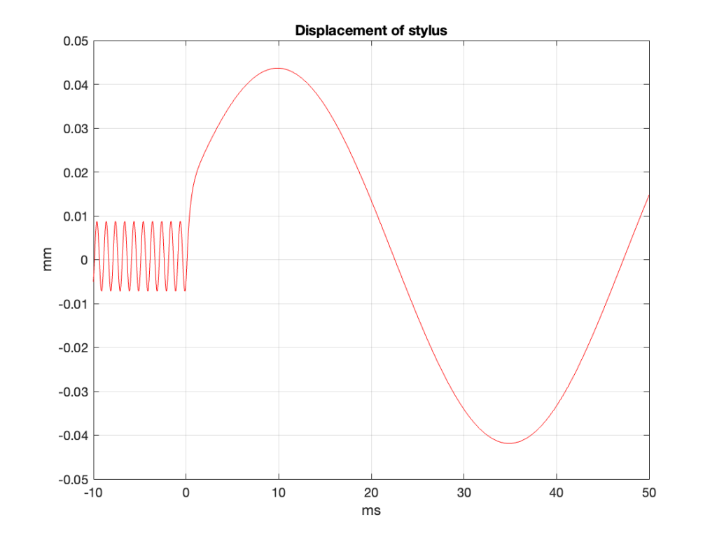
Back to the story: if we take the signal in Figure 10 and integrate it (and scale it – which isn’t really important for this discussion), we get the curve in Figure 11.
Figure 11
This gives us a good idea of the actual shape of the left wall of the groove in the vinyl for that particular signal.
So, as you can see there, if the connection between the cantilever and the pickup doesn’t have a high enough compliance, it’s no wonder that the needle gets thrown out of the record groove. That’s a heck of a bump to deal with! To be honest, it’s also a little amazing to me that the needle that’s behaving (like the one that produced the output shown in Figure 7) can actually put up with that kind of abuse.
(Special thanks to Jakob Dyreby for helping me to wrap my head around the simulation part of this posting. I did the math, but only after he pointed me in the right direction.)
Post script
Every once in a while, someone will send me a link to a YouTube page that shows an electron microscope “video” of a needle tracking a groove in a vinyl record. If you listen to the explanation of that video, he explains that it’s not really a video. It’s a series of photographs that he took, one by one, and then assembled into a video.
This means that, in that video, the needle isn’t really behaving like it does in real life when the vinyl is moving underneath it.
Imagine setting up a video camera on the side of the road, next to a small speed bump, and making a video of a car driving over it. You’d see that, as the car drives by, the wheels move up into the wheel wells and the car doesn’t get pushed upwards as much, since some of the vertical movement caused by the speed bump is “taken up” by the car’s springs and shock absorbers.
If, instead, you set up a camera, and got the car to move forwards 5 cm and stop – and you take a photo, then the car moves forwards another 5 cm and stops – and you take another photo, and the you repeat this until the car is out of the frame – and then you assemble all of those photos into a video, it would look very different. The car would not remain horizontal when the wheels are on the speed bump because the springs and shock absorbers wouldn’t be compressed at all.
That video is like the second “video” of the car. Of course, it’s still interesting, and it’s well-explained, so no one is playing any tricks on you. But it’s not a video of what actually happens…
This is just a collection of information about turntables and vinyl for anyone wanting to dig deeper into It (which might mean that it’s just for me…). I’ll keep adding to this (and completing it) as time goes by.
Glossary
Cantilever
The rod or arm that connects the stylus on one end to the “motor” on the other.
Effective Length
The straight-line distance between the pivot point of the tonearm and the top of the stylus
Equivalent Mass
definition to come
Flutter
Higher-frequency modulation of the audio frequency caused by changes in the groove speed. These may be the result of changes in problems such as unstable motor speed, variable compliance on a belt, issues with a spindle bearing, drive wheel eccentricity, and other issues.
Flutter describes a modulation in the groove speed ranging from 6 to 100 times a second (6 Hz to 100 Hz).
Frequency Drift
Very long-term (or low-frequency) changes in the audio frequency, typically caused by slow changes in the platter rotation speed.
Typically, changes with a modulation frequency of less than 0.5 Hz (a period of no less than 2 seconds) are considered to be frequency drift. Faster changes are labelled “Wow”
Groove
The v-shaped track pressed into the surface of the vinyl record, in which the stylus sits
Linear Tracking
A tonearm that moves linearly, following a path that is parallel to the radius line traced by the stylus. This (in theory) ensures that the tracking error is always 0º, however, in practice this error is merely small.
Modulation Width
The distance measured on a line through the spindle from the start of the modulated groove to the end of the modulated groove. This is approximately 3″ or 76 mm.
Mounting Distance
The distance between the spindle and the pivot point of the tonearm.
Needle
Also known as the stylus. The point that is placed in the groove of the vinyl record. Some persons distinguish between the “stylus” (to indicate the chisel on the mastering lathe that creates the groove in the master record), and the “needle” (to indicate the portion of the pickup on a turntable that plays the signal).
Null Radius
The radius (distance between the spindle and the stylus) where the tracking error is 0º. A typically-designed and correctly installed radial tracking tonearm has two null radii (see this posting).
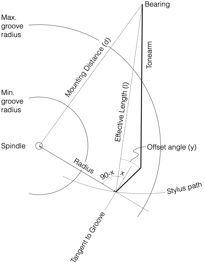
Offset Angle
The angle between the axis of the stylus and a line drawn between the tonearm pivot and the stylus. See the line diagram below.
Overhang
The difference between the Effective Length of the tonearm and the Mounting Distance. This value is used in some equations for calculating the Tracking Error.
Pickup, Electromagnetic
Includes three general types: Moving Coil, Moving Magnet, and Variable Reluctance (aka Moving Iron). These produce an output proportional to the velocity of the stylus movement.
Pickup, Piezoelectic
Produces an output proportional to the displacement of the stylus.
Pitch
The density of the groove count per distance in lines per inch or lines per mm. The pitch can vary from disc to disc, or even within a single track, according to the requirements of the mastering.
Radial Tracking
A tonearm that rotates on a pivot point with the stylus tracing a circular path around that pivot.
Radius
The distance between the centre of the vinyl disc and the pickup stylus.
RIAA
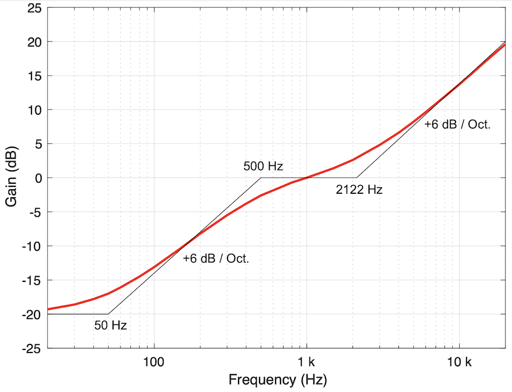
A pre-emphasis / de-emphasis filter designed to fill two functions.
The first is a high-frequency attenuation de-emphasis that reduces the playback system’s sensitivity to surface noise. This requires a reciprocal high-frequency pre-emphasis boost.
The second is a low-frequency attenuation pre-emphasis that maintains a constant modulation amplitude at lower frequencies to avoid over-excursion of the playback stylus. This requires a reciprocal low-frequency de-emphasis boost.
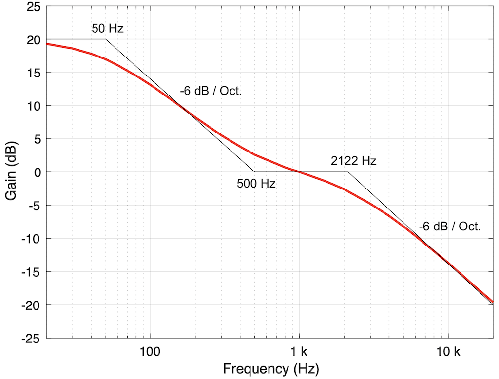
The first of the two plots below, show the theoretical (black lines) and typical (red) response of the pre-emphasis filter. The second of the two plots shows the de-emphasis filter response.
Side Thrust
definition to come
Skating Force
definition to come
Spindle
The centre of the platter around which the record rotates
Stylus
Also known as the needle. The point that is placed in the groove of the vinyl record. Some persons distinguish between the “stylus” (to indicate the chisel on the mastering lathe that creates the groove in the master record), and the “needle” (to indicate the portion of the pickup on a turntable that plays the signal).
Stylus, Bonded vs. Nude
Although the tip of the stylus is typically made of diamond today, in lower-cost units, that diamond tip is mounted or bonded to a metal pin (typically steel, aluminium, or titanium) which is, in turn, connected to the cantilever (the long “arm” that connects back to the cartridge housing). This bonded design is cheaper to manufacture, but it results in a high mass at the stylus tip, which means that it will not move easily at high frequencies.
In order to reduce mass, the metal pin is eliminated, and the entire stylus is made of diamond instead. This makes things more costly, but reduces the mass dramatically, so it is preferred if the goal is higher sound performance. This design is known as a nude stylus.
Tracking Error
The angle between the tangent to the groove and the alignment of the stylus. In a perfect system, the stylus would align with the tangent to the groove at all radii (distances from the spindle), since this matches the angular rotation of the cutting head when the master was made on a lathe. A linear tracking arm minimises this error. A radial tracking arm can be designed to have two radii with no tracking error (each called a “Null Radius”) but will have some measurable tracking error at all other locations on the disk.
One side-effect of tracking error is distortion of the audio signal, typically calculated and expressed as a 2nd-harmonic distortion on a sinusoidal audio signal. However, higher order distortion and intermodulation artefacts also exist.
Warp Wow
A modulation of the frequency of the audio signal caused by vertical changes in the vinyl surface (a warped record). This typically happens at a lower frequency, which is why it is “warp wow” and not “warp flutter”.
Wow
Low-frequency modulation of the audio frequency caused by changes in the groove speed. These may be the result of changes in problems such as rotation speed of the platter, discs with an incorrectly-placed centre hole, or vertical changes in the surface of the vinyl, and other issues.
Wow is a modulation in the groove speed ranging from once every 2 seconds to 6 times a second (0.5 Hz to 6 Hz). Note that, for a turntable, the rotational speed of the disc is within this range. (At 33 1/3 RPM: 1 revolution every 1.8 seconds is equal to approximately 0.556 Hz.)
Disk size limits
Outside starting diameter
7″ discs
6.78″, +0.06″, -0.00″
172.2 mm, +1.524 mm, – 0.0 mm
10″ discs
9.72″, +0.06″, -0.00″
246.9 mm, +1.524 mm, – 0.0 mm
12″ discs
11.72″, +0.06″, -0.00″
297.7 mm, +1.524 mm, – 0.0 mm
Start of modulated pitch diameter
7″ discs
6.63″, +0.00″, -0.03″
168.4 mm, +0.0 mm, – 0.762 mm
10″ discs
9.50″, +0.00″, -0.03″
241.3 mm, +0.0 mm, – 0.762 mm
12″ discs
11.50″, +0.00″, -0.03″
292.1 mm, +0.0 mm, – 0.762 mm
Minimum inside diameter
7″ discs
4.25″
107.95 mm
10″ discs
4.75″
120.65 mm
12″ discs
4.75″
120.65 mm
Lockout Groove diameter
7″ discs
3.88″, +0.00, -0.08
98.552 mm, +0.0 mm, -2.032 mm
10″ discs
4.19″, +0.00, -0.08
106.426 mm, +0.0 mm, -0.762 mm
12″ discs
4.19″, +0.00, -0.08
106.426 mm, +0.0 mm, -0.762 mm
Unmodulated (silent) groove width
2 mil minimum, 4 mil maximum
0.0508 mm minimum, 0.1016 mm maximum
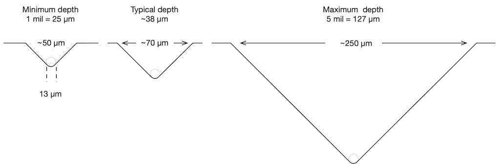
Modulated groove depth
1 mil minimum, 5 mil maximum
0.0254 mm minimum, 0.127 mm maximum
The figure below shows the typical, minimum, and maximum groove depths, drawn to scale (with a 13 µm spherical stylus)
Signal levels
A typical standard reference level is a velocity of 35.4 mm/sec on one channel.
This means that a monophonic signal (identical signal in both channels) with that modulation will have a lateral (side-to-side) velocity of 50 mm/sec.
Typically measured with a 3150 Hz sinusoidal tone, played from the vinyl surface
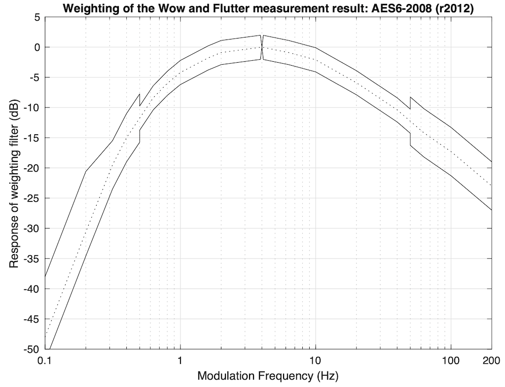
This signal is then de-modulated to determine its change over time. That modulation is then filtered through the response shown below which approximates human sensitivity to frequency modulation of an audio signal. More detailed information is given below
The AES6-2008 standard, which is the currently accepted method of measuring and expressing the wow and flutter specification, uses a “2σ” or “2-Sigma” method, which is a way of looking at the peak deviation to give a kind of “worst-case” scenario. In this method, the tone is played from a disc and captured for as long a time as is possible (or feasible). Firstly, the average value of the actual frequency of the output is found (in theory, it’s fixed at 3,150 Hz, but this is never true). Next, the short-term variation of the actual frequency over time is compared to the average, and weighted using the filter shown above. The result shows the instantaneous frequency variations over the length of the captured signal, relative to the average frequency (however, the effect of very slow and very fast changes have been reduced by the filter). Finally, the standard deviation of the variation from the average is calculated, and multiplied by 2 (hence “2-Sigma”, or “two times the standard deviation”), resulting in the value that is shown as the specification. The reason two standard deviations is chosen is that (in the typical case where the deviation has a Gaussian distribution) the actual Wow & Flutter value should exceed this value no more than 5% of the time.
References
All of these are available online. Some of them require you to purchase them (or be a member of an organisation).
“Tracking Angle in Phonograph Pickups” B. B. Bauer. Electronics magazine, March 1945
“Minimising Pickup Tracking Error” Dr. John D. Seagrave, Audiocraft Magazine, December 1956, January 1957, and August 1957
“Understanding Phono Cartridges” S.K. Pramanik, Audio magazine, March 1979
“Tonearm Geometry and Setup Demystified” Martin D. Kessler and B.V.Pisha, Audio magazine, January 1980
“Understanding Tonearms” S.K. Pramanik, Audio magazine, June 1980
“Analytic Treatment of Tracking Error and Notes on Optimal Pick-up Design” H.G.Baerwald, Journal of the Society of Motion Picture Engineers, December 1941
“Pickup Arm Design” J.K. Stevenson, Wireless World magazine, May 1966, and June 1966
“The Optimum Pivot Position on Tonearm” S. Takahashi et. al., Audio Engineering Society Preprint no. 1390 (61st Convention, November 1978)
“Audible Effects of Mechanical Resonances in Turntables” Brüel and Kjær Application Note (1977)
“Basic Disc Mastering”; “ Larry Boden (1981)
“Cartridge / Arm / Turntable Followup: Loose Ends and New Developments” The Audio Critic, 1:43 (Spring/Fall, 1978)
“Have Tone Arm Designers Forgotten Their High-School Geometry?” The Audio Critic, 1:31 (Jan./Feb. 1977).
“How the Stereo Disc Works” Radio-Electronics, (July 1958)
“Manual of Analogue Sound Restoration Techniques” Peter Copeland (2008)
“On the Mechanics of Tonearms” Dick Pierce (2005)
“Reproduction of Sound in High-Fidelity and Stereo Phonographs” Edgar Villchur (1966)
Journal of the Audio Engineering Society (www.aes.org)
“Centennial Issue: The Phonograph and Sound Recording After One-Hundred Years” Vol. 25, No. 10/11 (Oct./Nov. 1977)
“Factors Affecting the Stylus / Groove Relationship in Phonograph Playback Systems” C.R. Bastiaans; Vol. 15 Issue 4 (Oct. 1967)
“Further Thoughts on Geometric Conditions in the Cutting and Playing of Stereo Disk” C.R. Bastiaans; Vol. 11 Issue 1 (Jan. 1963)
“Record Changers, Turntables, and Tone Arms-A Brief Technical History” James H. Kogen; Vol. 25 (Oct./Nov. 1977)
“Some Thoughts on Geometric Conditions in the Cutting and Playing of Stereodiscs and Their Influence on the Final Sound Picture” Ooms, Johan L., Bastiaans, C. R.; Vol. 7 Issue 3 (Jul. 1959)
45 500: Hi-Fi Technics: Requirements for Disk Recording Reproducing Equipment
45 507: Measuring Apparatus for Frequency Variations in Sound Recording Equipment
45 538: Definitions for Disk Record Reproducing Equipment
45 539: Disk Record Reproducing Equipment: Directives for Measurements, Markings, and Audio Frequency, Connections, Dimensions of Interchangeable Pickups, Requirements of Playback Amplifiers
45 541: Frequency Test Record St 33 and M 33 (33 1/3 rev/min; Stereo and Mono)
45 542: Distortion Test Record St 33 and St 45 (33 1/3 or 45 rev/min; Stereo)
45 543: Frequency Response and Crosstalk Test Record
45 544: Rumble Measurement Test Record St 33 and M 33 (33 1/3 rev/min; Stereo and Mono)
45 545: Wow and Flutter Test Records, 33 1/3 and 45 rev/min
45 546: Stereophonic Disk Record St 45 (45 rpm)
45 547: Stereophonic Disk Record St 33 (33 1/3 rpm)
45 548 Aptitude for Performance of Disk Record Reproducing Equipment
45 549: Tracking Ability Test Record
IEC Publications
98: Recommendations for Lateral-Cut Commercial and Transcription Disk Recordings
98: Processed Disk Records and Reproducing Equipment
386: Method of Measurement of Speed Fluctuations in Sound Recording and Reproducing Equipment