B&O Tech: It’s not just a soundbar

#74 in a series of articles about the technology behind Bang & Olufsen loudspeakers

Bang & Olufsen recently released its latest television called BeoVision Eclipse. If you look around the web for comments and reviews, one of the things you’ll come across is that many people are calling it a “soundbar” which is only partly true, which is why B&O calls is a SoundCenter instead.

In order to explain the difference, let’s start by looking at what basic components you would need to buy in order to have the equivalent capabilities of the Eclipse.

  • 4K HDR OLED screen
  • Multichannel audio
    • Surround processor + Three-channel amplifier with 150 watts per channel OR
    • Audio-Video Receiver (AVR) with 150 watts per channel
    • 19 discrete audio output channels
    • 1- to 16.5- up/down mixing, dynamic with signal
    • User-configurable dynamic output routing
    • Intelligent Bass Management
  • Three full-range loudspeakers
  • DLNA, Streaming, and multiroom compatible

This is shown in the block diagram in Figure 1 – and it’s important to note that this just an overview of the capabilities – not a thorough list.

Fig 1. An overview of the basic components you would need to buy to get an equivalent of a BeoVision Eclipse.

I’m from the acoustics department, so I’m not going to talk about the video portion of the Eclipse – it’s best to stick with what I know…

Built-in loudspeakers

From the outside, the Eclipse obviously has 3 woofers, each driven by its own 100 W amplifier as well as 2  full range drivers and a tweeter, each of which is individually powered by its own 50 W amplifier. Those 6 amplifiers are each fed by its own Digital to Analogue Converter (or DAC).

The total result of this is a discrete 3-channel loudspeaker array (which some might label a “soundbar”) that is fully-active, and with all processing (such as crossovers, filtering, and ABL, as described in this posting) performed in the Digital Signal Processing (or DSP).

When it leaves the factory, those three channels are preset to act as the Left Front (Lf), Centre Front (Cf), and Right Front (Rf) audio channels, however, these can be changed by the user, as I’ll describe below.

External loudspeakers

The BeoVision Eclipse, like all other current BeoVision televisions includes both wired and wireless outputs for connection to external loudspeakers for customers who either want to have a larger multichannel system, or wish to have the option to upgrade to one in the future.

The Eclipse has 8 wired outputs (on 4 Power Link connections – each of which has 2 discrete audio channels) and 8 wireless outputs (using Wireless Power Link).

This means that, in total, you can have up to 19 loudspeakers delivering signals in a large multichannel surround system (8 wired + 8 wireless + 3 internal). However, even if you have all of those loudspeakers connected, you don’t have to use all of them all of the time…

Audio signal processing

There are many Surround Processors and Audio-Video Receivers (or AVR’s) in the world. These have the primary job of receiving a signal (say, from an HDMI input) and decoding it, splitting it up into the video and audio outputs. The audio channels in the signal are then sent to the appropriate output. However, with almost all Surround Processors and AVRs, the output channel routing is fixed. In other words, the left surround output of the AVR always goes to the same loudspeaker, in the left surround position.

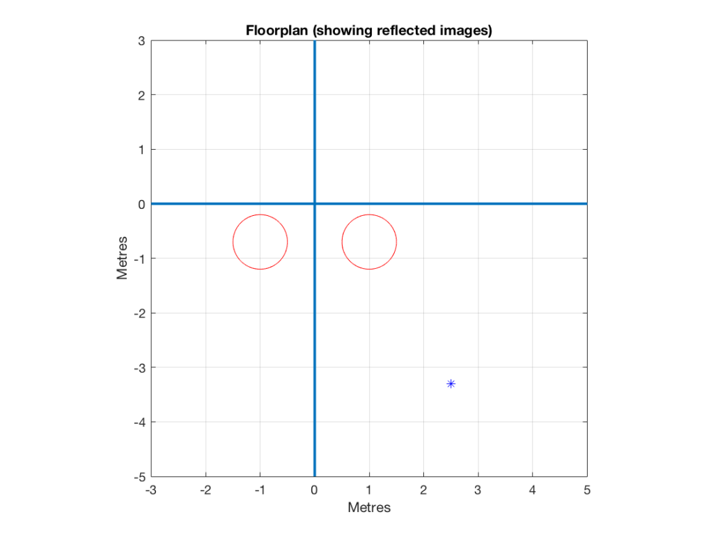
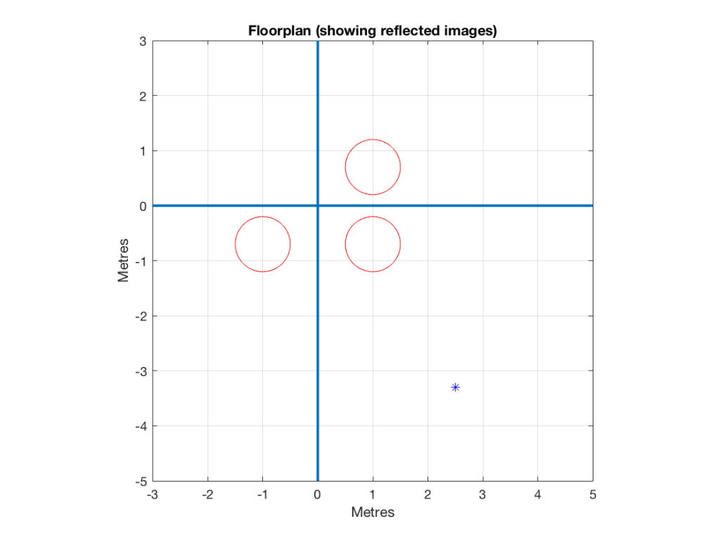
In a Bang & Olufsen television like the BeoVision Eclipse, this routing is not fixed. So, for example, if you connect two extra external loudspeakers, you might choose to use them as the Left Surround (Ls) and Right Surround (Rs) outputs, with the three internal loudspeakers providing the Lf, Cf, and Rf channels. This is shown in Figure 2.

Fig 2. An example of a 5-channel surround system made with a BeoVision Eclipse, providing the front three channels, and two external loudspeakers acting as the Left and Right Surrounds.

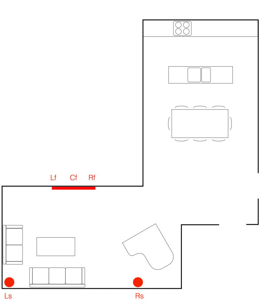
This configuration would be saved as a “Speaker Preset” and labelled as you wish (for example, “surround sound”) and even set as a default configuration for the inputs that you wish (the Blu-ray player, for example).

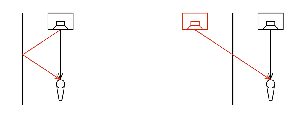
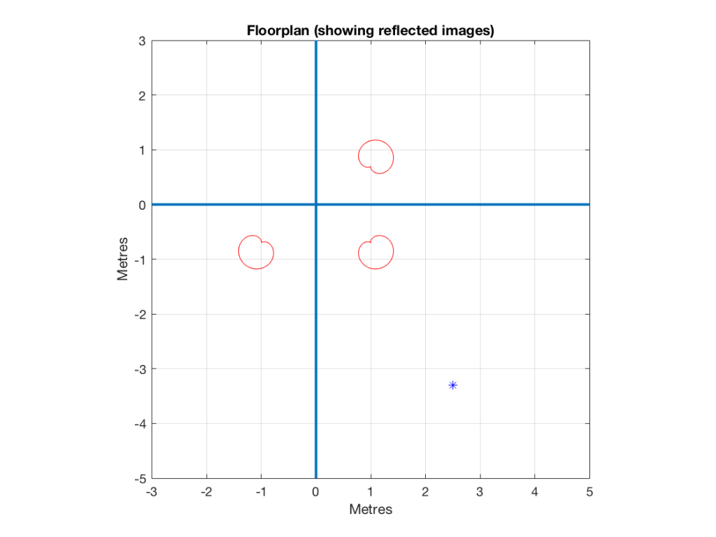
However, you aren’t stuck with this setup. Let’s say, for example, that, when you have dinner, you would like to use the external loudspeakers ONLY as a stereo pair, as is shown below in Figure 3.

Fig 3. The same system, reconfigured to act as a stereo pair for background music while dining.

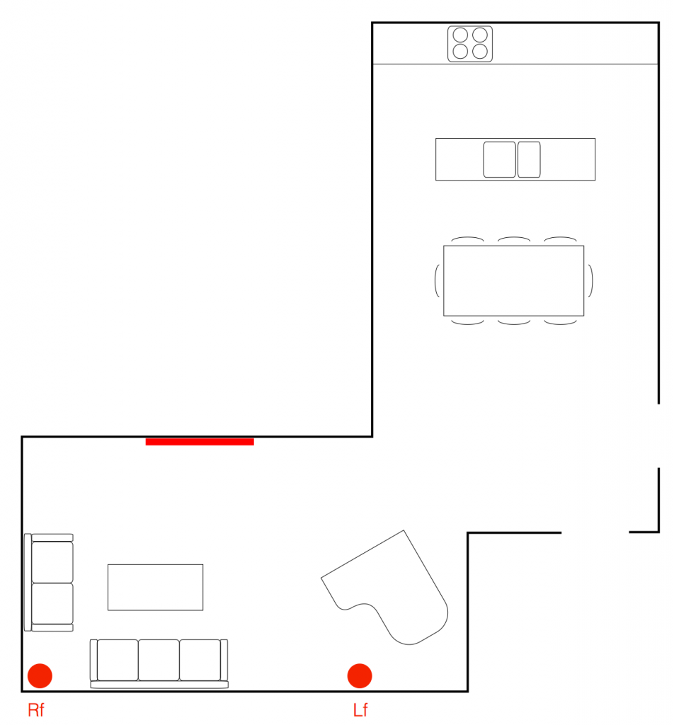
Now, the external loudspeakers have changed their Speaker Roles. They were Left Surround and Right Surround in Figure 2 – but now they’re Right Front and Left Front. This configuration can be saved as another Speaker Group, and labelled something like “Dinner Music” for example.

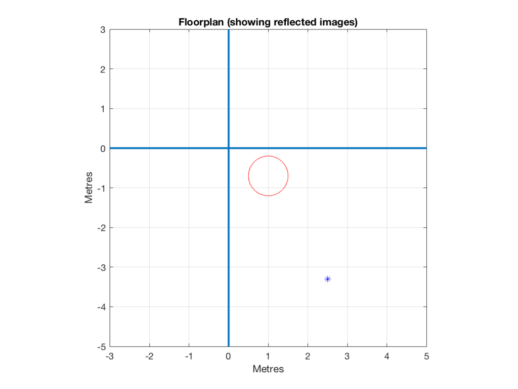
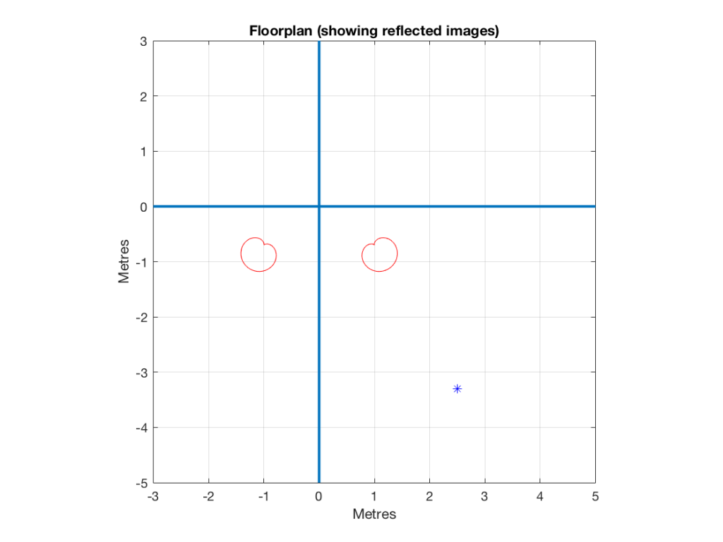
You could also do something completely non-intuitive – for example a configuration for watching the evening news, where you only need to hear the dialogue, but everyone else in the house is either asleep, or not interested in current affairs. Then you can route the Centre Front channel to the closet loudspeaker only, as shown below in Figure 4.

Fig 4. A non-intuitive Speaker Group for listening to late-night evening news without disturbing the rest of the house.

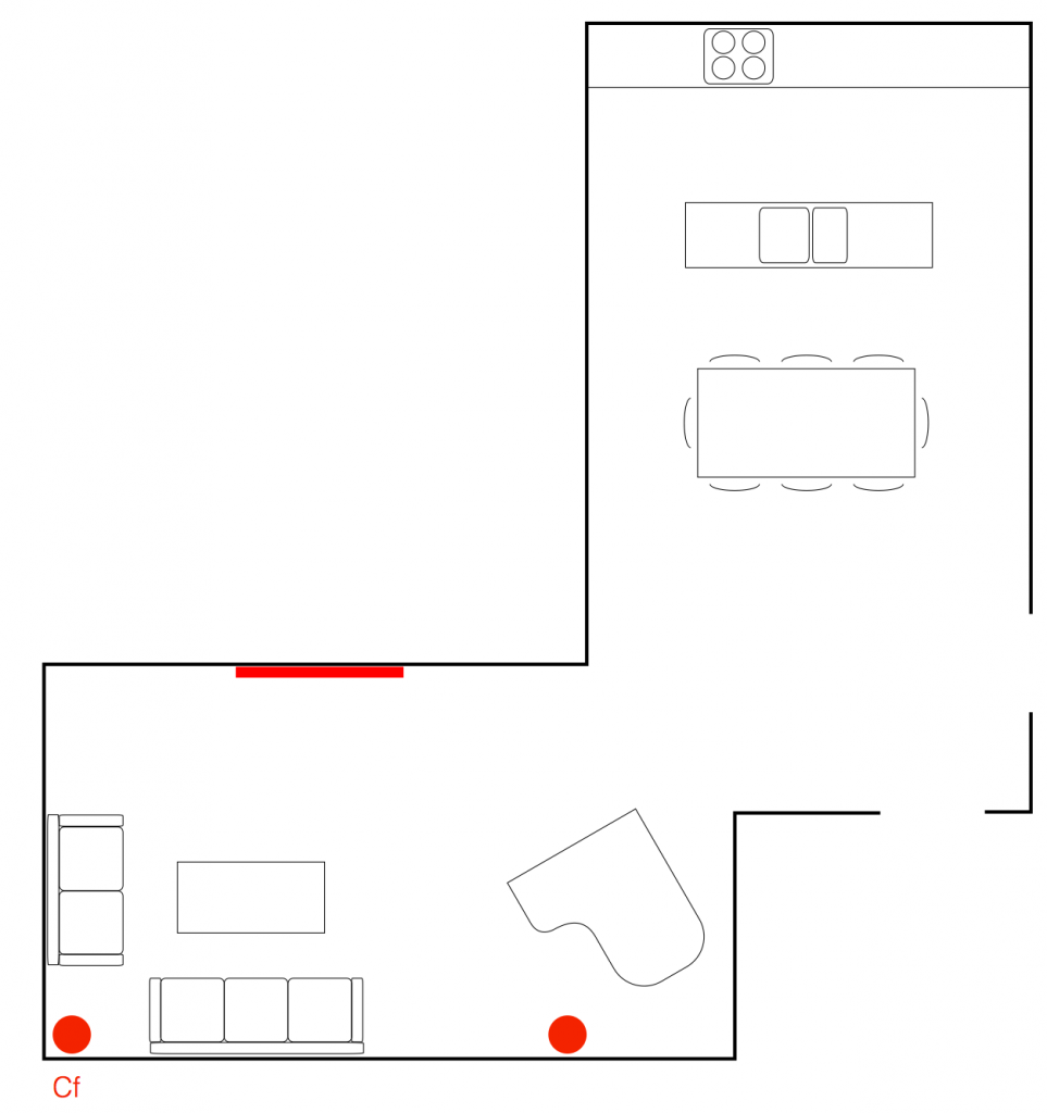
This can be saved as another Speaker Group, called “Speech – Night Listening” for example.

It should also be noted that there are no rules applied to the distribution of Speaker Roles in a Speaker Group. So, for example, if you wanted to have 19 loudspeakers, all playing the Left Surround channel, the TV will let you do this. I’m not suggesting that this is a good idea – I’m merely saying that the TV will not stop you from doing this…

Of course, when you create a Speaker Group, you not only define the various roles of the loudspeakers, you also set their Speaker Levels and Speaker Distances to ensure that the levels and time-of-arrivals are all aligned as you require for your configuration.

Update: I just made a new Speaker Group on a system with a BeoVision Eclipse and a pair of BeoLab 90’s that I thought might make an interesting addition to this section. The Eclipse Speaker Group was created such that all connected loudspeakers (internal and external) were set to have a Speaker Role of NONE. This basically means that the TV uses no loudspeakers. You may wonder why this is a useful Speaker Group. The reason is that I was using the Eclipse as an external monitor for a computer, but I wanted to listen to music from the BeoLab 90’s from another device (which is connected to their S/P-DIF Coaxial input). So, the Eclipse turns off the BeoLab 90’s, which “frees them up” to automatically switch to the S/P-DIF input.


Up-/down-mixing capabilities

Internally, the Eclipse, like the BeoVision 11, Avant, Horizon, and 14, can create up to a 16-channel upmix of all signals that come into it, using the True Image algorithm. However, if your input channel mapping matches your output, then the upmixer does nothing. This decision (whether to upmix, downmix, or do nothing)  is continually made on-the-fly. So, for example, let’s say that you have a 5.1-channel loudspeaker configuration with 5 main loudspeakers and one subwoofer. You start by playing 2-channel  stereo music from a USB stick and the True Image algorithm will upmix the 2 input channels to your 5 output channels, and also bass mange the low frequency content to the subwoofer. You then switch to watch a DVD with a 5.1-channel signal, and True Image will connect the 6 input channels to the 6 loudspeakers directly without doing any interim spatial processing. Then, you change to a Blu-ray disc with 7.1-channel audio content and True Image will downmix the 8 incoming channels to your 6 loudspeakers.

All of this happens automatically, and is also true if you switch Speaker Groups. So, if you start watching the 5.1-channel DVD with a 5.1-channel Speaker Group, then True Image will pass the signals through. If you then switch to the 2-channel Speaker Group, True Image will automatically start downmixing for you (rather than just not playing the “missing” output channels).

Of course, if you’re a purist, then the True Image algorithm can be disabled, and the incoming audio channels can be just routed to their respective outputs directly. However, this means that if your input format does not match your output format, then either you’ll not hear some audio channels (if you have more input channels than output channels) OR some loudspeakers will not play audio (if you have fewer input channels than output channels).

Intelligent bass management

If all of the external loudspeakers that you’ve connected to the BeoVision Eclipse are Bang & Olufsen products, then you simply tell the television which loudspeaker models you have (if they’re connected wirelessly, then this happens automatically) and the TV will automatically decide whether each loudspeaker should be bass-managed or not. This is because the TV is programmed with the bass capabilities of all Bang & Olufsen loudspeakers in the current portfolio – and many legacy products. This means that the TV “knows” which speakers can play the loudest bass – so it will automatically configure itself for each Speaker Group, ensuring that your bass is re-routed to the most capable loudspeakers.

Of course, this can be over-ridden in the user menus. So, if you wish to disable Bass Management, you can do so. However, you can also create extreme cases where you send the bass managed signal to all loudspeakers. This is not necessarily a good idea – nor will it necessarily give you the most bass (due to possible phase differences between the loudspeakers, for example) – however, you can do it if you wish.

If the external loudspeakers are not Bang & Olufsen products, then you simply choose “Other” as your Speaker Connection (or speaker type) in the menus, and the TV will know that it cannot make automatic decisions about the bass management – so you’ll have to configure this yourself.

Automatic Latency Management

Different Bang & Olufsen loudspeakers have different “latencies”. (The latency of a loudspeaker is the time it takes for the signal to go through it – from the electrical input to the acoustical output.) For some older products (like the BeoLab 3, for example) then the latency is 0 ms, because it is an analogue loudspeaker. For some others, it is between 2.5 and 5 ms (depending on the particular loudspeaker). The BeoLab 50 and BeoLab 90 each have two latency modes: either 25 ms or 100 ms, depending on how they are configured.

In order to ensure that all of these different loudspeakers can “live together” in a single surround system (and also in a multiroom configuration with other products in your house), the TV must also “know” the latencies of the various loudspeakers that are connected to it.

In addition, the BeoVision Eclipse can “tell” the BeoLab 50 and 90 to change latency settings on-the-fly to optimise the configuration to ensure lip sync. (Note that, in order for this to happen, the BeoLab 50 and 90 must be set to “Auto” latency mode, allowing them to be switched by the TV.)


Other Features

As I said at the top, I’m concentrating on the audio and acoustic features of the BeoVision Eclipse. There are many aspects of the LG screen that I won’t discuss here. In addition, there are a multitude of video and audio input options and built-in sources (like Netflix, Amazon, Google Chromecast, Apple AirPlay, and so on…) which I also won’t go through.

Finally, of course, it goes without saying that in order to control all of this you only need to have one remote control sitting on your coffee table…

For more information

True Image Upmixing

What’s So Great About Active Loudspeakers?


B&O Tech: Directivity and Reflections

#73 in a series of articles about the technology behind Bang & Olufsen loudspeakers

The setup

Let’s start by inventing a loudspeaker. It has a perfectly flat on-axis response in a free field. This means that if you send a signal into it, then it doesn’t cause any particular frequency to sound louder or quieter than the others when you measure it in an infinite space that is free of reflections.

We’ll also say that it has a perfectly omnidirectional directivity. This means that the loudspeaker has the same behaviour in all directions – there is no “front” or “back” – sound goes everywhere identically.

Let’s then put that loudspeaker in a strange room that has only two walls – the left wall and the front wall – and these extend to infinity. We’ll put the loudspeaker, say 1 m from the left wall and 70 cm from the front wall. These are completely arbitrary values, but they’re not weird… Finally, we’ll sit 3 m away from the loudspeaker, as if we were set up to listen to it as the left front loudspeaker in a stereo pair.

A floorpan of that setup is shown below in Figure 1.

Fig 01: The centre of the red circle shows the location of the loudspeaker, and the circle itself represents the fact that the loudspeaker is omnidirectional. The blue lines are the walls, and the blue asterisk is the listening position.

If the two walls were completely absorptive, then there would be no energy reflected from them. If we were to replace the loudspeaker with a light bulb, then the equivalent would be to paint the walls flat black so no light would be reflected. In this theoretically perfect case, then the impulse response and the magnitude response of the loudspeaker at the listening position would be the same as in a free field, since there are no reflections. These would look like the plots in Figure 2.

Fig 2. The impulse response and the magnitude response of the arrangement shown in Figure 1. Note that it takes approximately 9 ms for the sound to reach the listening position, and that there are no reflections after that. The magnitude response is completely flat, but has an overall gain of almost -10 dB since it is measured relative to a reference distance of 1 m.


Through the looking glass

Imagine that you’re standing outdoors on a moonless night, and the only things you have with you are a lightbulb (that is magically lit) and a mirror. You’ll be able to see two light bulbs – the real one, and the one that is reflected by the mirror. If there is really no other light and no other objects, then you won’t even know that it’s a mirror, and you’ll just see two light bulbs (unless, of course, you can see yourself as well…)

In 1929, an acoustical physicist working at Bell Laboratories named Carl F. Eyring presented a new idea to the Acoustical Society of America. He was trying to calculate the reverberation time in “dead” rooms by considering that the walls were perfect mirrors, and that instead of thinking of sound sources and reflections, you could just pretend that the walls didn’t exist, and that the reflections were actually just images of other sound sources on the other side of the wall (just like that second light bulb in the example above…)

Fig 3: Two conceptual diagrams showing (in a perfect world) identical systems. On the left is the direct sound (the black arrow) and the reflected sound (the red arrow) reaching the microphone. On the right, we see the direct sound coming from the “real” loudspeaker, and the reflection coming from an image of that loudspeaker on the other side of the wall – as if the wall were not there.

This method of simulating and predicting acoustical behaviour in rooms, now called the “image model” has been used by many people over the decades. Eyring published a paper describing it in 1930, but it has since been standard method, both for prediction and acoustical simulation (first proposed by Allen and Berkley in 1979).


The effects of one sidewall reflection

Let’s use the image model to do a very basic prediction of what will happen to our impulse and magnitude responses if we have a single reflection from the left-hand wall.

Fig 4: An image model representation of the same loudspeaker shown in Figure 1, with a perfectly reflective sidewall on the left.
Fig. 5:The Impulse response and magnitude response of the resulting signal at the listening position. Notice that the direct sound is identical to that shown in Figure 2, but now there is an additional reflection that arrives about 5 ms later, and quieter, since the path the reflection takes is longer. The resulting magnitude response is a classic “comb filter”, so-called because it looks like a hair comb if you plot it on a linear frequency scale.

As can be seen in Figure 5, the resulting magnitude response of an omnidirectional loudspeaker with a single, perfect reflection certainly has some noticeable artefacts. If the listening position were closer to the loudspeaker, the artefacts would be smaller, since the reflected signal would be quieter than the direct sound The further away you get, the more the two path lengths are the same, and therefore the bigger the effect on the summed signal.

Of course, this is an unrealistic simulation, since everything is “perfect” – perfect reflection, perfectly omnidirectional loudspeaker with a perfectly flat magnitude response, and so on… However, for the purposes of this posting, that’s good enough.

Let’s now change the directivity of the loudspeaker to alter the balance of level between the direct and the reflected sounds. We’ll make the loudspeaker’s beam width more narrow, giving it the same behaviour as a cardioid microphone (which is called a cardioid because a polar plot of its directivity pattern looks like a heart – cardiovascular and cardioid have the same root).

Fig. 6: The same arrangement as shown in Figure 4, but with more directional loudspeakers.
Fig. 7: The impulse and magnitude responses of the arrangement shown in Figure 6.

If you look at Figure 7, you’ll see that the times of arrival of the two signals have not changed, but that the effect of the artefact in the frequency domain is reduced (the peaks and dips are smaller). The frequencies of the peaks and dips are the same as in Figure 5 because those are determined by the delay difference between the two spikes in the impulse response. The peaks and dips are smaller because the reflected sound is quieter (because the image loudspeaker – the reflected signal is beaming in a different direction).

Let’s try a different directivity pattern – a dipole, which has a polar patter than looks like a figure “8”.

Fig 8: A dipole loudspeaker and its image, in the same positions as in Figure 4.
Fig 9: The impulse and magnitude responses of the arrangement shown in Figure 8.

Notice now that, because the listening position is almost perfectly in line with the “null” – the “dead zone” of the reflected loudspeaker, there is almost nothing to reflect. Consequently, there is very little effect on the on-axis magnitude response of the loudspeaker, as can be seen in the magnitude response in Figure 9.

So, the moral of the story so far is that without moving the loudspeaker or the listening position, or changing the wall’s characteristics, the time response and magnitude response of the loudspeaker at the listening position is heavily dependent on the loudspeaker’s directivity.


Two reflections

Let’s continue the experiment, making the front wall reflective as well.

Fig 10: An image model representation of two reflections and an omnidirectional loudspeaker.


Fig 11. The impulse and magnitude responses at the listening position with two reflections and an omnidirectional loudspeaker, as shown in Figure 10. Note that the second impulse (the first reflection after the direct sound) is the one from the front wall, since that image is closer to the listening position.


Fig 12. An image model representation of two reflections and a loudspeaker with a cardioid directivity.


Fig 13. The artefacts on the magnitude response are considerably less for a cardioid loudspeaker than with an omnidirectional, since, as can be seen, the reflected signals are considerably quieter due to the angle of the listening position with respect to the rotation of the image loudspeakers.


Fig 14: An image model representation of two reflections and a loudspeaker with a dipole directivity.


Fig 15: The artefacts on the magnitude response are different when the loudspeaker is a dipole. Notice that the sidewall reflection is much quieter than the front wall reflection, as we saw already in Figure 9.

In Figure 15, one additional effect can be seen. Since the reflection off the front wall is negative (in other words, it “pulls” when the direct sound “pushes”) due to the behaviour of the dipole, there is a cancellation in the low frequencies, causing a drop in level in the low end. If we were to push the loudspeaker closer to the front wall, this effect would become more and more obvious.


The moral of the story is…

Of course, this is all very theoretical, however, it should give you an idea of three things.

The first is a simple method of thinking about reflections. You can use the Image Model method to imagine that your walls are mirrors, and you can “see” the other loudspeakers on the other sides of those mirrors. Those images are where your reflections are coming from.

The second is the obvious point – that the summed magnitude response of a loudspeaker’s direct sound, and its reflections is dependent on many things, the directivity being one of them.

The third is possibly the most important. All three of the loudspeaker models I’ve used here have razor-flat on-axis responses in a free field. So, if you were trying to decide which of these three loudspeakers to buy, you’d look at their “frequency response” plots or data and see that all of them are flat to within 0.0001 dB from 1 Hz to infinity Hz, and you’d think that they’d all sound “the same” under the same conditions. However, nothing could be further from the truth. These three loudspeaker with identical on-axis responses will sound completely different. This does not mean that an on-axis magnitude response is useless. It only means that it’s useless in the absence of other information such as the loudspeaker’s power response or its frequency-dependent directivity.

To keep things simple, I have not included frequency-dependent directivity effects. I may do that some day – but beware that it is not enough to say “the loudspeaker beams at higher frequencies so I don’t have to worry about it up there” because that’s not necessarily true – it’s different from loudspeaker to loudspeaker.

This also means that none of the plots I’ve shown here can be used to conclude anything about the real world. All it’s good for is to get a conceptual, intuitive idea of what’s going on when you put a loudspeaker near a wall.

One final comment: the microphone that I’m simulating here has an omnidirectional characteristic. This means that it is as sensitive to the reflected sound as it is to the direct sound, since the angle of incidence of the sound is irrelevant. The way we humans perceive sound is different. We do not perceive the comb filter that the microphone sees when the reflection is coming in from our side, since this is information that is recognised by the brain as being reflected – and it’s used to determine the distance to the sound source. However, if you plug one ear, you may notice that things sound more like you see in the plots, since you lose part of your ability to localise the direction of the signals in the horizontal plane.


For more reading…

Allen, J.B., & Berkley, D.A. (1979) “Image Method for Efficiently Simulating Small-Room Acoustics,” Journal of the Acoustical Society of America, 65(4): 943-950, April.

Eyring, C.F. (1930) “Reverberation Time in ‘Dead’ Rooms,” Journal of the Acoustical Society of America, 1: 217-241.

Gibbs, B.M., & Jones, D.K., (1972) “A Simple Image Method for Calculating the Distribution of Sound Pressure Levels Within an Enclosure,” Acustica, 26: 24-32.


B&O Tech: Signal Mixing and Decomposition

#72 in a series of articles about the technology behind Bang & Olufsen loudspeakers

After a previous posting, someone posted this as part of a comment:

“What I’ve been asking myself for a long time: how does a single driver manage to produce two or more frequencies (or a frequency range) at the exact same time? For example a singer singing while the guitar plays in the background. Could you try to explain how this works?”

So, this posting is an attempt to answer that question.


Adding signals together

Sound is a change of air pressure over time. That pressure is modulating on top of the day’s average barometric pressure – which is just a measurement of how closely the air particles around you are squeezed together. On a high-pressure day, the air is more densely packed – on a low pressure day, the air is less dense.

When you make a sound, you make slight variations in that pressure – so, for example, when a woofer moves out of a loudspeaker enclosure (a fancy name for “box”) then it pushes the air particles in front of it, and they’re squeezed together, resulting in a compression wave that radiates away from the loudspeaker. When the woofer pulls into the enclosure, it pulls the air particles apart, and you get a rarefaction wave instead. (You can see an animation of this at this posting.)

Let’s make a graph that shows a plot of the acoustic pressure changing over time. This is shown below in Figure 1. When this plot shows a positive number, it means that the air particles are being compressed more than normal. When it’s negative, then they’re being separated more than normal. Without getting into too many details, let’s just say that this is a low frequency. (If you want to get picky, then you’ll see that this is one cycle of a wave that takes 100 ms. Since there are 1000 ms in a second, then this must be a 10 Hertz signal, because 1000 / 100 = 10. That makes it a VERY low frequency by normal audio standards… )

Figure 1. A low frequency signal.

Let’s also look at an example of a higher frequency, shown in Figure 2, below.

Figure 2: A signal with a higher frequency and a lower amplitude than the one shown in Figure 1.

We can see that Figure 2 has a higher frequency signal, because it moves up and down more frequently. It has 5 cycles (5 ‘ups’ and ‘downs’) in the same amount of time that it took the wave in Figure 1 to have 1 cycle – therefore it is 5 times the frequency (and therefore, if you’re being picky, 50 Hz – which, by audio standards, is also a very low frequency, but this is just an example…)

Ignoring that ACTUAL frequencies that are plotted there, let’s pretend for a moment that the low frequency (Figure 1) came from a bass guitar and the higher frequency (Figure 2) came from a singer. If we took those two signals and put them into a mixing console, what does the result look like?

Well, we take the instantaneous value of the signal at one moment in time and add it to the instantaneous value of the other signal at the same time. Let’s do that.

Figure 3: Some details on the signal in Figure 1.

Figure 3 shows the same signal as in Figure 1, but I’ve pointed out the values at two moments in time – at 25 ms and at 50 ms. So, for example, you can see there that, at 25 ms, the value is 0.5 – whatever that means…

Figure 4: Some details on the signal in Figure 2.

Figure 4 shows the same signal as in Figure 2, but I’ve pointed out the values at two same moments in time – at 25 ms and at 50 ms. So, for example, you can see there that, at 25 ms, the value is 0.1 – whatever that means.

We take the value at 25 ms from each of the two signals (0.5 and 0.1) and add them together to get 0.6. This is the value of the signal at the output of the mixer at 25 ms. At 50 ms, the mixer’s output will have a value of 0 (because 0+0 = 0). This is shown graphically below for all of the values of both plots from 0 ms to 100 ms.

Figure 5: The result of adding Figures 1 and 2.

So, you can see in Figure 5 what the result will be. This signal contains both the low frequency, shown in Figure 1 and the higher frequency shown in Figure 2. If we send this combined signal to a loudspeaker, then both signals will get reproduced.

One interesting thing to note is that this mixing can also be done in the air. If a bass guitar and a singer are performing a song together, live, then the bass is pushing and pulling the molecules at the same time that the singer’s voice does. So, if at 25 ms, the bass pushes the molecules with a value of 0.5 (whatever that means) and the singer pushes the molecules with a value of 0.1, then your eardrum will be pushed in with a value of 0.6.  So, the summation of the pressure signals happens in the air, just like it does as voltages or voltage measurements in the mixing console.


Splitting signals apart

Typically, however, a loudspeaker is comprised of more than one driver – for example, a woofer (for the low frequencies) and a tweeter (for the high frequencies). (Of course, some loudspeakers have more than two drivers, but we’re keeping things simple today…)

So, what we do there is to put the total signal, shown in Figure 5, and send it to two circuits that change how loud things are, depending on their frequency. One circuit is called a “low pass filter” because it allows low frequencies to pass through it unchanged, but it reduces the level of higher frequencies. The other circuit is called a “high pass filter” because it allows the high frequencies to pass through it unchanged, but it reduces the level of the lower frequencies. (we won’t talk about how those circuits do that in this posting…)

We can plot the two characteristics of these two circuits – an example of which is shown in Figure 6.

Figure 6: An example of the gains applied to a signal by a low pass filter (in red) and a high pass filter (in black). Notice that, at one frequency, both filters have the same output level. That frequency is called the “crossover frequency” because it’s the frequency where the two filters’ responses cross over each other.

IF we send a signal like the one in Figure 5 to a crossover that happens to have a crossover frequency that is between the two frequencies it contains, then the signal will be split into two – one output containing mostly low-frequency components, and the other one containing mostly high-frequency components. Examples of these are shown below.

Figure 7: An example of the output of the signal from Figure 5, sent though a low-pass filter. Notice that it looks a lot like Figure 1 (the low frequency component of the combined signal) – but there’s a little bit of Figure 2 (the high frequency component) left in there…


Figure 8: An example of the output of the signal from Figure 5, sent though a high-pass filter. Notice that it looks a lot like Figure 2 (the high frequency component of the combined signal) – but there’s a little bit of Figure 1 (the low frequency component) left in there…


NB: Of course, everything I’ve shown here are just examples to make the concept intuitive. The crossover shown in Figure 6 would not work the way I’ve shown it in Figures 7 and 8 because the crossover frequency is too high compared to the 10 Hz and 50 Hz waves that I used in the example. So, please do not make comments talking about how I chose the wrong crossover frequency…


B&O Tech: BeoLab 50’s Beam Width Control

#65 in a series of articles about the technology behind Bang & Olufsen loudspeakers

Although active Beam Width Control is a feature that was first released with the BeoLab 90 in November of 2015, the question of loudspeaker directivity has been a primary concern in Bang & Olufsen’s acoustics research and development for decades.

As a primer, for a history of loudspeaker directivity at B&O, please read the article in the book downloadable at this site. You can read about the directivity in the BeoLab 5 here, or about the development Beam Width Control in BeoLab 90 here and here.

Bang & Olufsen has just released its second loudspeaker with Beam Width Control – the BeoLab 50. This loudspeaker borrows some techniques from the BeoLab 90, and introduces a new method of controlling horizontal directivity: a moveable Acoustic Lens.

Fig 1: BeoLab 50 PT1. The “PT” stands for ProtoType. This was the very first full-sized working model of the BeoLab 50, assembled from parts made using a 3D printer.

The three woofers and three midrange drivers of the BeoLab 50 (seen above in Figure 1) are each driven by its own amplifier, DAC and signal processing chain. This allows us to create a custom digital filter for each driver that allows us to control not only its magnitude response, but its behaviour both in time and phase (vs. frequency). This means that, just as in the BeoLab 90, the drivers can either cancel each other’s signals, or work together, in different directions radiating outwards from the loudspeaker. This means that, by manipulating the filters in the DSP (the Digital Signal Processing) chain, the loudspeaker can either produce a narrow or a wide beam of sound in the horizontal plane, according to the preferences of the listener.

Fig 2: Horizontal directivity of the BeoLab 50 in Narrow mode. Contour lines are in steps of 3 dB and are normalised to the on-axis response.


Fig 3: Horizontal directivity of the BeoLab 50 in Wide mode. Contour lines are in steps of 3 dB and are normalised to the on-axis response.


You’ll see that there is only one tweeter, and it is placed in an Acoustic Lens that is somewhat similar to the one that was first used in the BeoLab 5 in 2002. However, BeoLab 50’s Acoustic Lens is considerably different in a couple of respects.

Firstly, the geometry of the Lens has been completely re-engineered, resulting in a significant improvement in its behaviour over the frequency range of the loudspeaker driver. One of the obvious results of this change is its diameter – it’s much larger than the lens on the tweeter of the BeoLab 5. In addition, if you were to slice the BeoLab 50 Lens vertically, you will see that the shape of the curve has changed as well.

However, the Acoustic Lens was originally designed to ensure that the horizontal width of sound radiating from a tweeter was not only more like itself over a wider frequency range – but that it was also quite wide when compared to a conventional tweeter. So what’s an Acoustic Lens doing on a loudspeaker that can also be used in a Narrow mode? Well, another update to the Acoustic Lens is the movable “cheeks” on either side of the tweeter. These can be angled to a more narrow position that focuses the beam width of the tweeter to match the width of the midrange drivers.


Fig 4: Acoustic Lens in “narrow” mode on a later prototype of the BeoLab 50. You can see that this is a prototype, since the disc under the lens does not align very well with the top of the loudspeaker.


In Wide Mode, the sides of the lens open up to produce a wider radiation pattern, just as in the original Acoustic Lens.

Fig 5: Acoustic Lens in “wide” mode on a later prototype of the BeoLab 50. You can see that this is a prototype, since the disc under the lens does not align very well with the top of the loudspeaker.


So, the BeoLab 50 provides a selectable Beam Width, but does so not only “merely” by changing filters in the DSP, but also with moving mechanical components.

Of course, changing the geometry of the Lens not only alters the directivity, but it changes the magnitude response of the tweeter as well – even in a free field (a theoretical, infinitely large room that is free of reflections). As a result, it was necessary to have a different tuning of the signal sent to the tweeter in order to compensate for that difference and ensure that the overall “sound” of the BeoLab 50 does not change when switching between the two beam widths. This is similar to what is done in the Active Room Compensation, where a different filter is required to compensate for the room’s acoustical behaviour for each beam width. This is because, at least as far as the room is concerned, changing the beam width changes how the loudspeaker couples to the room at different frequencies.