Category: acoustics
Immersive audio
Typical Errors in Digital Audio: Wrapping up
This “series” of postings was intended to describe some of the errors that I commonly see when I measure and evaluate digital audio systems. All of the examples I’ve shown are taken from measurements of commercially-available hardware and software – they’re not “beta” versions that are in development.
There are some reasons why I wrote this series that I’d like to make reasonably explicit.
- Many of the errors that I’ve described here are significant – but will, in some cases, not be detected by “typical” audio measurements such as frequency response or SNR measurements.
- For example, the small clicks caused by skip/insert artefacts will not show up in a SNR or a THD+N measurement due to the fact that the artefacts are so small with respect to the signal. This does not mean that they are not audible. Play a midrange sine tone (say, in the 2 -3 kHz region… nothing too annoying) and listen for clicks.
- As another example, the drifting time clock problems described here are not evident as jitter or sampling rate errors at the digital output of the device. These are caused by a clocking problems inside the signal path. So, a simple measurement of the digital output carrier will not, in any way, reveal the significance of the problem inside the system.
- Aliasing artefacts (described here) may not show up in a THD measurement (since aliasing artefacts are not Harmonic). They will show up as part of the Noise in a THD+N measurement, but they certainly do not sound like noise, since they are weirdly correlated with the signal. Therefore you cannot sweep them under the rug as “noise”…
- Some of the problems with some systems only exist with some combinations of file format / sampling rate / bit depth, as I showed here. So, for example, if you read a test of a streaming system that says “I checked the device/system using a 44.1 kHz, 16-bit WAV file, and found that its output is bit-perfect” Then this is probably true. However, there is no guarantee whatsoever that this “bit-perfect-ness” will hold for all other sampling rates, bit depths, and file formats.
- Sometimes, if you test a system, it will behave for a while, and then not behave. As we saw in Figure 10 of this posting, the first skip-insert error happened exactly 10 seconds after the file started playing. So, if you do a quick sweep that only lasts for 9.5 seconds you’ll think that this system is “bit-perfect” – which is true most of the time – but not all of the time…
- Sometimes, you just don’t get what you’ve paid for – although that’s not necessarily the fault of the company you’re paying…
Unfortunately, the only thing that I have concluded after having done lots of measurements of lots of systems is that, unless you do a full set of measurements on a given system, you don’t really know how it behaves. And, it might not behave the same tomorrow because something in the chain might have had a software update overnight.
However, there are two more thing that I’d like to point out (which I’ve already mentioned in one of the postings).
Firstly, just because a system has a digital input (or source, say, a file) and a digital output does not guarantee that it’s perfect. These days the weakest links in a digital audio signal path are typically in the signal processing software or the clocking of the devices in the audio chain.
Secondly, if you do have a digital audio system or device, and something sounds weird, there’s probably no need to look for the most complicated solution to the problem. Typically, the problem is in a poor implementation of an algorithm somewhere in the system. In other words, there’s no point in arguing over whether your DAC has a 120 dB or a 123 dB SNR if you have a sampling rate converter upstream that is generating aliasing at -60 dB… Don’t spend money “upgrading” your mains cables if your real problem is that audio samples are being left out every half second because your source and your receiver can’t agree on how fast their clocks should run.
So, the bad news is that trying to keep track of all of this is complicated at best. More likely impossible.
On the other hand, if you do have a system that you’re happy with, it’s best to not read anything I wrote and just keep listening to your music…
B&O Tech: Airtight excuses
#79 in a series of articles about the technology behind Bang & Olufsen loudspeakers
“Love at first sight? Let me just put on my glasses.”
Ljupka Cvetanova, The New Land
When I’m working on the sound design for a new pair of (over-ear, closed) headphones, I have to take off my glasses (which makes it difficult for me to see my computer screen…) I’ll explain.
Let’s over-simplify and consider a block diagram of a closed (and therefore “over-ear”) headphone, sitting on one side of your head. This is represented by Figure 1.

One of the important things to note there is that the air in the chamber between the headphone diaphragm and the ear canal is sealed from the outside world.
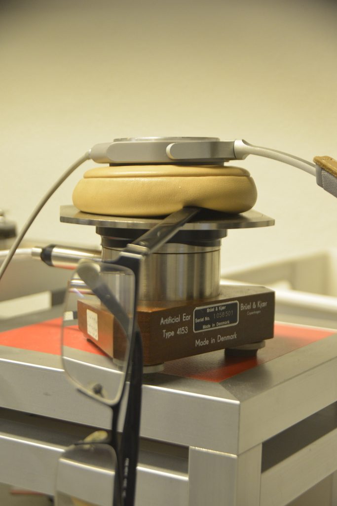
So, if I put such a headphone on an artificial ear (which is a microphone in a small hole in the middle of a plate – it is remarkably well-represented by the red lines in Figure 1….) I can measure its magnitude response. I’ll call this the “reference”. It doesn’t matter to me what the measurement looks like, since this is just a magnitude response which is the combination of the headphone’s response and the artificial ear’s response – with some incorrect positioning thrown into the mix.

If I then remove the headphones from the plate, and put them back on, in what I think is the same position, and then do the measurement again, I’ll get another curve.
Then, I’ll subtract the “reference measurement” (the first one) from the second measurement to see what the difference is. An example of this is plotted in Figure 2.

Now, let’s consider what happens when the seal is broken. I’ll stick a small piece of metal (actually an Allan key, or a hex wrench, depending on where you live) in between the headphones and the plate, causing a leak in the air between the internal cavity and the outside world, as shown in Figure 4.


We then repeat the measurement, and subtract the original Reference measurement to see what happened. This is shown in Figure 6.
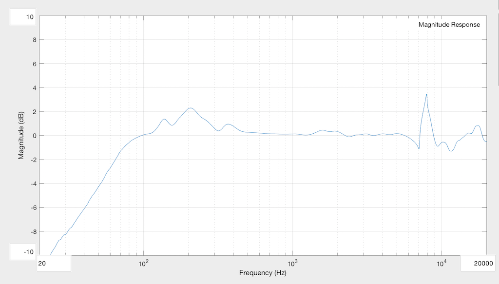
As you can see, the leak in the system causes us to lose bass, primarily. In the very low end, the loss is significant – more than 10 dB down at 20 Hz! Basically, what we’ve done here is to create an acoustical high-pass filter. (I’m not going to go into the physics of why this happens… That’s too much information for this posting.) You can also see that there’s a bump around 200 Hz which is also a result of the leak. The sharp peak up at 8 kHz is not caused by the leak – it’s just an artefact of the headphones having moved a little on the plate when I put in the Allen Key.
Now let’s make the leak bigger. I’ll stick the arm of my glasses in between the plate and the leather pad.
The result of this measurement (again with the Reference subtracted) is shown in Figure 8.

Now you can see that the high pass filter’s cutoff frequency has risen, and the resonance in the system has not only increased in frequency (to 400 Hz or so) but also in magnitude (to almost +10 dB! Again, the sharp wiggles at the top are mostly just artefacts caused by changes in position…
Just to check and see that I haven’t done something stupid, I’ll remove the glasses, and run the measurement again…

The result of this measurement is shown in Figure 10.

So, there are a couple of things to be learned here…
Firstly, if you and a friend both listen to the same pair of closed, sealed headphones, and you disagree about the relative level of bass, check that you’re both not wearing glasses or large earrings…
The more general interpretation of that previous point is that small leaks in the system have a big effect on the response of the headphones in the low-frequency region. Those leaks can happen as a result of many things – not just the arm of your glasses. Hair can also cause the problem. Or, for example, if the headphones are slightly big, and/or your head is slightly small, then the area where your jaw meets your neck under your pinna (around your mastoid gland) is one possile place for leaks. This can also happen if you have a very sharp corner around your jaw (say you are Audrey Hepburn, for example), and the ear cup padding is stiff. Interestingly, as time passes, the foam and covering soften and may change shape slightly to seal these leaks. So, as the headphones match the shape of your head over time, you might get a better seal and a change in the bass level. This might be interpreted by some people as having “broken in” the headphones – but what you’ve actually done is to “break in” the padding so that it fits your head better.
Secondly, those big, sharp spikes up the high end aren’t insignificant… They’re the result of small movements in the headphones on the measuring system. A similar thing happens when you move headphones on your head – but it can be even more significant due to effects caused by your pinna. This is why, many people, when doing headphone measurements, will do many measurements (say, 5 to 10) and average the results. Those errors in placement are not just the result of shifts on the plate – they may also be caused by differences in “clamping pressure” – so, if I angled the headphones a little on that table, then they might be pressing harder on the artificial ear, possibly only on one side of the ear cup, and this will also change the measured response in the high frequency bands.

Of course, it’s possible to reduce this problem by making the foam more compliant (a fancy word for “squishy”) – which may, in turn, mean that the response will be more different for different users due to different head widths. Or the problem could be reduced by increasing the clamping force, which will in turn make the headphones uncomfortable because they’re squeezing your head. Or, you could embrace the leak, and make a pair of open headphones – but those will not give you much passive noise isolation from the outside world. In fact, you won’t have any at all…
So as you can see, as a manufacturer, this issue has to be balanced with other issues when designing the headphones in the first place…
Or you can just take off your glasses, close your eyes, and listen…
Addendum
Please don’t jump too far in your conclusions as a result of seeing these measurements. You should NOT interpret them to mean that, if you wear glasses, you will get a 10 dB bump at 400 Hz. The actual response that you will get from your headphones depends on the size of the leak, the volume of the chamber in the ear cup (which is partly dependent on the size of your pinna, since that occupies a significant portion of the volume inside the chamber) and other factors.
The take-home message here is: when you’re evaluating a pair of closed, over-ear headphones: small leaks have an effect on the low frequency response, and small changes in position have an effect on the high-frequency response. The details of those effects are almost impossible to predict accurately.
Typical Errors in Digital Audio: Part 2 – Dither
Reminder: This is still just the lead-up to the real topic of this series. However, we have to get some basics out of the way first…
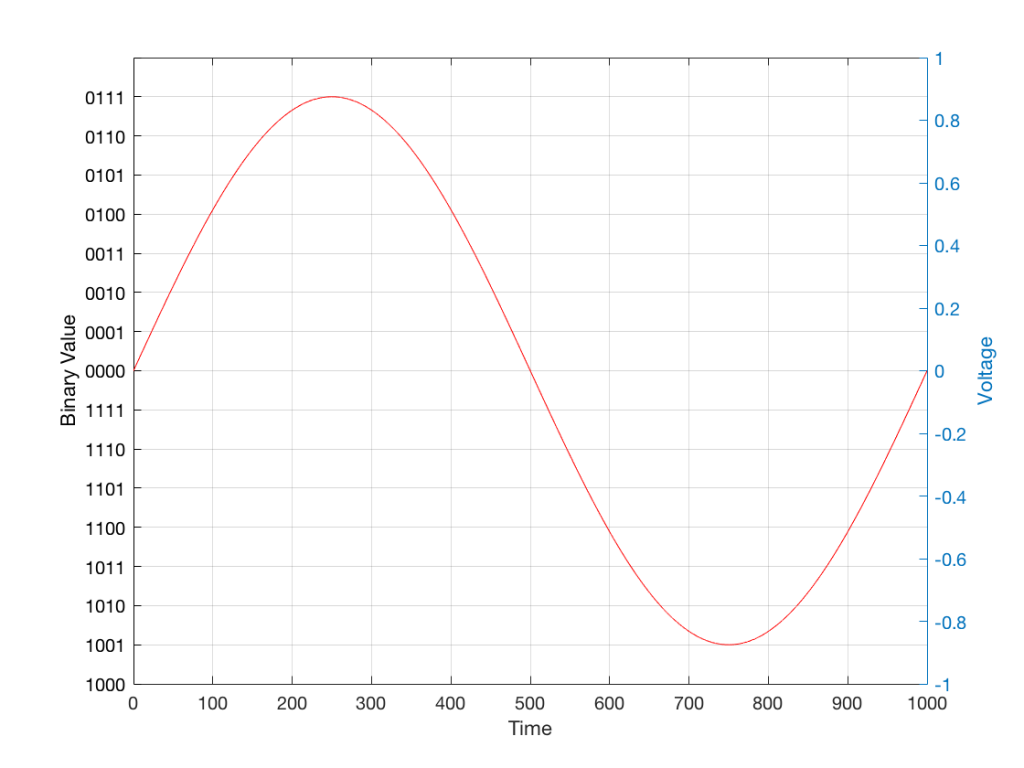
In the last posting, I talked about digital audio (more accurately, Linear Pulse Code Modulation or LPCM digital audio) is basically just a string of stored measurements of the electrical voltage that is analogous to the audio signal, which is a change in pressure over time…
For now, we’ll say that each measurement is rounded off to the nearest possible “tick” on the ruler that we’re using to measure the voltage. That rounding results in an error. However, (assuming that everything is working correctly) that error can never be bigger than 1/2 of a “step”. Therefore, in order to reduce the amount of error, we need to increase the number of ticks on the ruler.
Now we have to introduce a new word. If we really had a ruler, we could talk about whether the ticks are 1 mm apart – or 1/16″ – or whatever. We talk about the resolution of the ruler in terms of distance between ticks. However, if we are going to be more general, we can talk about the distance between two ticks being one “quantum” – a fancy word for the smallest step size on the ruler.
So, when you’re “rounding off to the nearest value” you are “quantising” the measurement (or “quantizing” it, if you live in Noah Webster’s country and therefore you harbor the belief that wordz should be spelled like they sound – and therefore the world needz more zees). This also means that the amount of error that you get as a result of that “rounding off” is called “quantisation error“.
In some explanations of this problem, you may read that this error is called “quantisation noise”. However, this isn’t always correct. This is because if something is “noise” then is is random, and therefore impossible to predict. However, that’s not strictly the case for quantisation error. If you know the signal, and you know the quantisation values, then you’ll be able to predict exactly what the error will be. So, although that error might sound like noise, technically speaking, it’s not. This can easily be seen in Figures 1 through 3 which demonstrate that the quantisation error causes a periodic, predictable error (and therefore harmonic distortion), not a random error (and therefore noise).
Sidebar: The reason people call it quantisation noise is that, if the signal is complicated (unlike a sine wave) and high in level relative to the quantisation levels – say a recording of Britney Spears, for example – then the distortion that is generated sounds “random-ish”, which causes people to just to the conclusion that it’s noise.
Now, let’s talk about perception for a while… We humans are really good at detecting patterns – signals – in an otherwise noisy world. This is just as true with hearing as it is with vision. So, if you have a sound that exists in a truly random background noise, then you can focus on listening to the sound and ignore the noise. For example, if you (like me) are old enough to have used cassette tapes, then you can remember listening to songs with a high background noise (the “tape hiss”) – but it wasn’t too annoying because the hiss was independent of the music, and constant. However, if you, like me, have listened to Bob Marley’s live version of “No Woman No Cry” from the “Legend” album, then you, like me, would miss the the feedback in the PA system at that point in the song when the FoH engineer wasn’t paying enough attention… That noise (the howl of the feedback) is not noise – it’s a signal… Which makes it just as important as the song itself. (I could get into a long boring talk about John Cage at this point, but I’ll try to not get too distracted…)
The problem with the signal in Figure 2 is that the error (shown in Figure 3) is periodic – it’s a signal that demands attention. If the signal that I was sending into the quantisation system (in Figure 1) was a little more complicated than a sine wave – say a sine wave with an amplitude modulation – then the error would be easily “trackable” by anyone who was listening.
So, what we want to do is to quantise the signal (because we’re assuming that we can’t make a better “ruler”) but to make the error random – so it is changed from distortion to noise. We do this by adding noise to the signal before we quantise it. The result of this is that the error will be randomised, and will become independent of the original signal… So, instead of a modulating signal with modulated distortion, we get a modulated signal with constant noise – which is easier for us to ignore. (It has the added benefit of spreading the frequency content of the error over a wide frequency band, rather than being stuck on the harmonics of the original signal… but let’s not talk about that…)
For example…
Let’s take a look at an example of this from an equivalent world – digital photography.
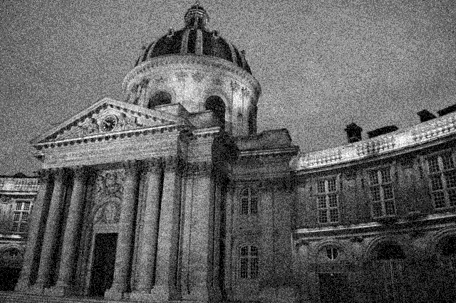
The photo in Figure 4 is a black and white photo – which actually means that it’s comprised of shades of gray ranging from black all the way to white. The photo has 272,640 individual pixels (because it’s 640 pixels wide and 426 pixels high). Each of those pixels is some shade of gray, but that shading does not have an infinite resolution. There are “only” 256 possible shades of gray available for each pixel.
So, each pixel has a number that can range from 0 (black) up to 255 (white).

If we were to zoom in to the top left corner of the photo and look at the values of the 64 pixels there (an 8×8 pixel square), you’d see that they are:
86 86 90 88 87 87 90 91
86 88 90 90 89 87 90 91
88 89 91 90 89 89 90 94
88 90 91 93 90 90 93 94
89 93 94 94 91 93 94 96
90 93 94 95 94 91 95 96
93 94 97 95 94 95 96 97
93 94 97 97 96 94 97 97
What if we were to reduce the available resolution so that there were fewer shades of gray between white and black? We can take the photo in Figure 1 and round the value in each pixel to the new value. For example, Figure 5 shows an example of the same photo reduced to only 4 levels of gray.

Now, if we look at those same pixels in the upper left corner, we’d see that their values are
102 102 102 102 102 102 102 102
102 102 102 102 102 102 102 102
102 102 102 102 102 102 102 102
102 102 102 102 102 102 102 102
102 102 102 102 102 102 102 102
102 102 102 102 102 102 102 102
102 102 102 102 102 102 102 102
102 102 102 102 102 102 102 102
They’ve all been quantised to the nearest available level, which is 102. (Our possible values are restricted to 0, 51, 102, 154, 205, and 255).
So, we can see that, by quantising the gray levels from 256 possible values down to only 6, we lose details in the photo. This should not be a surprise… That loss of detail means that, for example, the gentle transition from lighter to darker gray in the sky in the original is “flattened” to a light spot in a darker background, with a jagged edge at the transition between the two. Also, the details of the wall pillars between the windows are lost.
If we take our original photo and add noise to it – so were adding a random value to the value of each pixel in the original photo (I won’t talk about the range of those random values…) it will look like Figure 6. This photo has all 256 possible values of gray – the same as in Figure 1.

If we then quantise Figure 6 using our 6 possible values of gray, we get Figure 7. Notice that, although we do not have more grays than in Figure 5, we can see things like the gradual shading in the sky and some details in the walls between the tall windows.
That noise that we add to the original signal is called dither – because it is forcing the quantiser to be indecisive about which level to quantise to choose.
I should be clear here and say that dither does not eliminate quantisation error. The purpose of dither is to randomise the error, turning the quantisation error into noise instead of distortion. This makes it (among other things) independent of the signal that you’re listening to, so it’s easier for your brain to separate it from the music, and ignore it.
Addendum: Binary basics and SNR
We normally write down our numbers using a “base 10” notation. So, when I write down 9374 – I mean
9 x 1000 + 3 x 100 + 7 x 10 + 4 x 1
or
9 x 10³ + 3 x 10² + 7 x 101 + 4 x 100
We use base 10 notation – a system based on 10 digits (0 through 9) because we have 10 fingers.
If we only had 2 fingers, we would do things differently… We would only have 2 digits (0 and 1) and we would write down numbers like this:
11101
which would be the same as saying
1 x 16 + 1 x 8 + 1 x 4 + 0 x 2 + 1 x 1
or
1 x 24 + 1 x 23 + 1 x 22 + 0 x 21 + 1 x 20
The details of this are not important – but one small point is. If we’re using a base-10 system and we increase the number by one more digit – say, going from a 3-digit number to a 4-digit number, then we increase the possible number of values we can represent by a factor of 10. (in other words, there are 10 times as many possible values in the number XXXX than in XXX.)
If we’re using a base-2 system and we increase by one extra digit, we increase the number of possible values by a factor of 2. So XXXX has 2 times as many possible values as XXX.
Now, remember that the error that we generate when we quantise is no bigger than 1/2 of a quantisation step, regardless of the number of steps. So, if we double the number of steps (by adding an extra binary digit or bit to the value that we’re storing), then the signal can be twice as “far away” from the quantisation error.
This means that, by adding an extra bit to the stored value, we increase the potential signal-to-error ratio of our LPCM system by a factor of 2 – or 6.02 dB.
So, if we have a 16-bit LPCM signal, then a sine wave at the maximum level that it can be without clipping is about 6 dB/bit * 16 bits – 3 dB = 93 dB louder than the error. The reason we subtract the 3 dB from the value is that the error is +/- 0.5 of a quantisation step (normally called an “LSB” or “Least Significant Bit”).
Note as well that this calculation is just a rule of thumb. It is neither precise nor accurate, since the details of exactly what kind of error we have will have a minor effect on the actual number. However, it will be close enough.
Typical Errors in Digital Audio: Part 1
Introduction
Once upon a time, when I was a young whipper snapper, studying how to be a recording engineer (which is half of being a tonmeister) I had a textbook on sound recording. There were chapters in there on musical instruments, acoustics, microphones, mixing consoles, magnetic tape, and so on.. There was also a section on something called “digital audio” – but it was a portion of the chapter titled “Noise Reduction”.
Fast-forward a couple of years to 1983 and a new technology hit the market called “Compact Disc” (Here’s a fun fact for impressing people at your next dinner party: The “c” at the end of “disc” means it’s an optical medium. If it were magnetic, it would be a “disk”. So: Compact Disc, but Hard Disk.) Back then, the magazine advertisement read “Perfect Sound. Forever.” Then it hit the real world and the complaints started rolling in from people who believed that they knew things about audio. Some of these complaints were valid, and some were less so… Many of the ones that were valid no longer are, but it’s difficult to un-do a first impression.
Nowadays, it is very likely that almost-all-to-all of the music you listen to has been digital at some point in its life. Even if you’re listening to vinyl, it should not surprise you to know that the master version of the recording you’re hearing was probably stored on a hard disk or passed through a digital mixing console – or at least some of the tracks included some kind of digital processing (say, a guitar pedal or a reverb unit, for example). (I know, I know… There are exceptions. However, if you want to send me anti-digital hate mail you may not do it using a digital communication format such as e-mail. Use an analogue pen to write out your words on a piece of paper and send it to me by post. I look forward to receiving your analogue letters.)
Nowadays, a big part of my “day job” is to test (digital) audio systems to find out what’s wrong with them. So, I thought it would be interesting to do a series of postings that describe the typical kinds of errors that I look for (and find) when I’m digging down into the details.
In order to do this, I’m going to start by being a little redundant and describe the basics of how audio is converted from an analogue signal to a digital one – and hopefully address some of the misconceptions that are associated with this conversion process.
A quick introduction to sound
At the simplest level, sound can be described as a small change in air pressure (or barometric pressure) over short periods of time. If you’d like to have a better and more edu-tain-y version of this statement with animations and pretty colours, you could take 10 minutes to watch this video, for example.
That change in pressure can be “captured” by using a microphone, that is (at the simplest level) a device that has a change in air pressure at its input and a change in electrical voltage at its output. Ignoring a lot of details, we could say that if you were to plot a measurement of the air pressure (at the input of the microphone) over time, and you were to compare it to a plot of the measurement of the voltage (at the output of the microphone) over time, you would see the same curve on the two graphs. This means that the change in voltage is analogous to the change in air pressure.
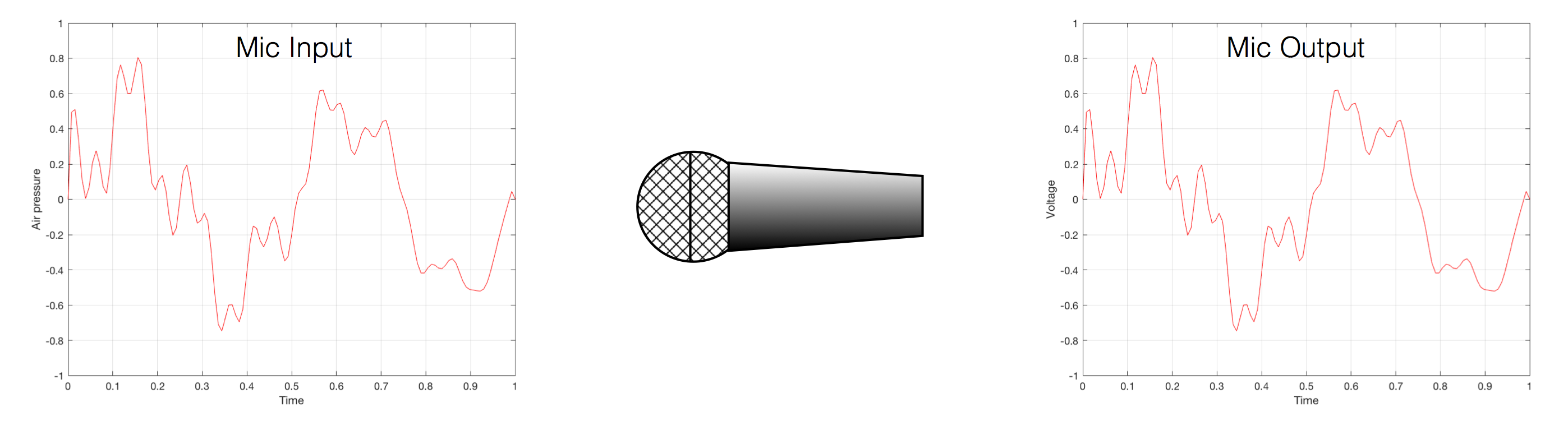
At this point in the conversation, I’ll make a point to say that, in theory, we could “zoom in” on either of those two curves shown in Figure 1 and see more and more details. This is like looking at a map of Canada – it has lots of crinkly, jagged lines. If you zoom in and look at the map of Newfoundland and Labrador, you’ll see that it has finer, crinkly, jagged lines. If you zoom in further, and stand where the water meets the shore in Trepassey and take a photo of your feet, you could copy it to draw a map of the line of where the water comes in around the rocks – and your toes – and you would wind up with even finer, crinkly, jagged lines… You could take this even further and get down to a microscopic or molecular level – but you get the idea… The point is that, in theory, both of the plots in Figure 1 have infinite resolution, both in time and in air pressure or voltage.
Now, let’s say that you wanted to take that microphone’s output and transmit it through a bunch of devices and wires that, in theory, all do nothing to the signal. Let’s say, for example, that you take the mic’s output, send it through a wire to a box that makes the signal twice as loud. Then take the output of that box and send it through a wire to another box that makes it half as loud. You take the output of that box and send it through a wire to a measuring device. What will you see? Unfortunately, none of the wires or boxes in the chain can be perfect, so you’ll probably see the signal plus something else which we’ll call the “error” in the system’s output. We can call it the error because, if we measure the input voltage and the output voltage at any one instant, we’ll probably see that they’re not identical. Since they should be identical, then the system must be making a mistake in transmitting the signal – so it makes errors…
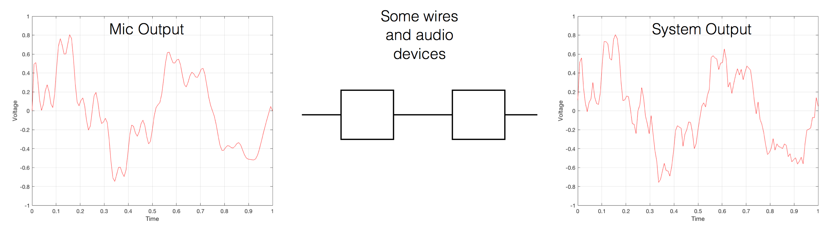
Pedantic Sidebar: Some people will call that error that the system adds to the signal “noise” – but I’m not going to call it that. This is because “noise” is a specific thing – noise is random – so if it’s not random, it’s not noise. Also, although the signal has been distorted (in that the output of the system is not identical to the input) I won’t call it “distortion” either, since distortion is a name that’s given to something that happens to the signal because the signal is there. (We would probably get at least some of the error out of our system even if we didn’t send any audio into it.) So, we could be slightly geeky and adequately vague and call the extra stuff “Distortion plus noise” but not “THD+N” – which stands for “Total Harmonic Distortion Plus Noise” – because not all kinds of distortion will produce a harmonic of the signal… but I’m getting ahead of myself…
So, we want to transmit (or store) the audio signal – but we want to reduce the noise caused by the transmission (or storage) system. One way to do this is to spend more money on your system. Use wires with better shielding, amplifiers with lower noise floors, bigger power supplies so that you don’t come close to their limits, run your magnetic tape twice as fast, and so on and so on. Or, you could convert the analogue signal (remember that it’s analogous to the change in air pressure over time) to one that is represented (and therefore transmitted or stored) digitally instead.
What does this mean?
Conversion from analogue to digital and back
(but skipping important details)
IMPORTANT: If you read this section, then please read the following postings as well. This is because, in order to keep things simple to start, I’m about to leave out some important details that I’ll add afterwards. However, if you don’t add the details, you could (understandably) jump to some incorrect conclusions (that many others before you have concluded…) So, if you don’t have time to read both sections, please don’t read either of them.
In the example above, we made a varying voltage that was analogous to the varying air pressure. If we wanted to store this, we could do it by varying the amount of magnetism on a wire or a coating on a tape, for example. Or we could cut a wiggly groove in a bit of vinyl that has a similar shape to the curve in the plots in Figure 1. Or, we could do something else: we could get a metronome (or a clock) and make a measurement of the voltage every time the metronome clicks, and write down the measurements.
For example, let’s zoom in on the first little bit of the signal in the plots in Figure 1
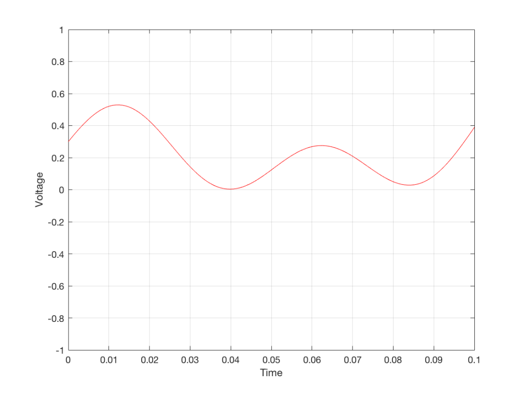
We’ll then put on a metronome and make a measurement of the voltage every time we hear the metronome click…
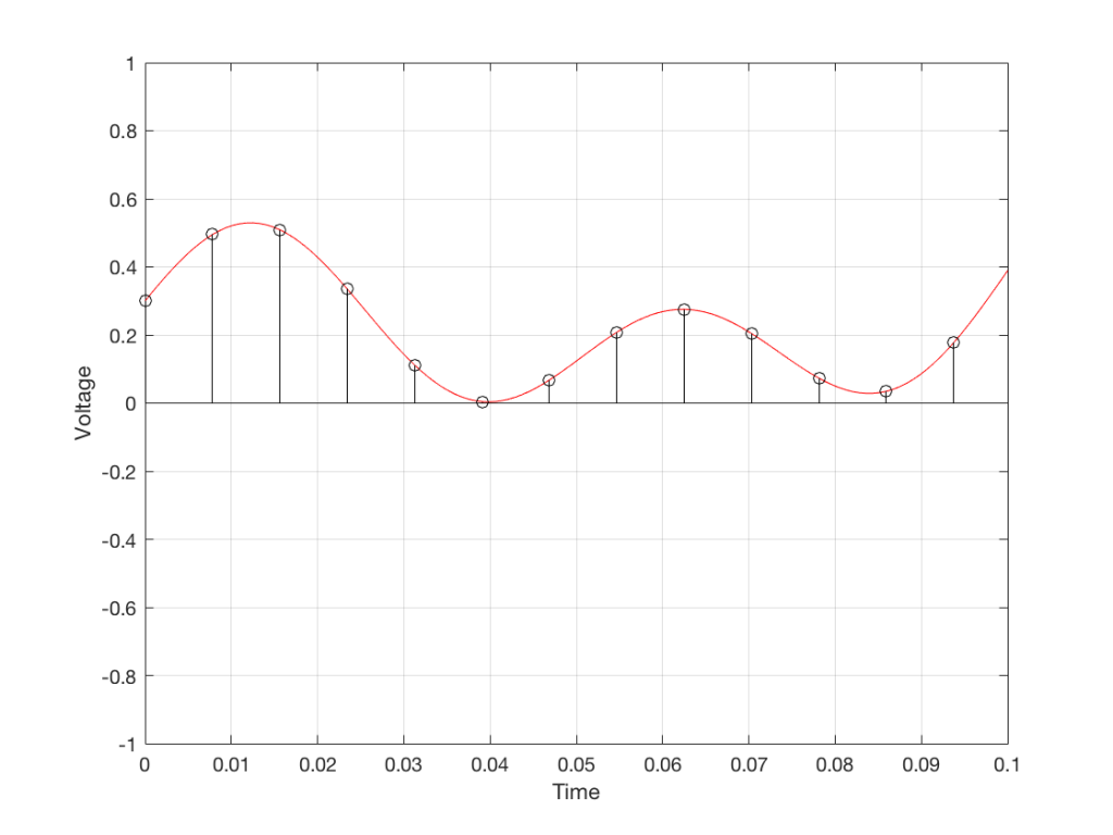
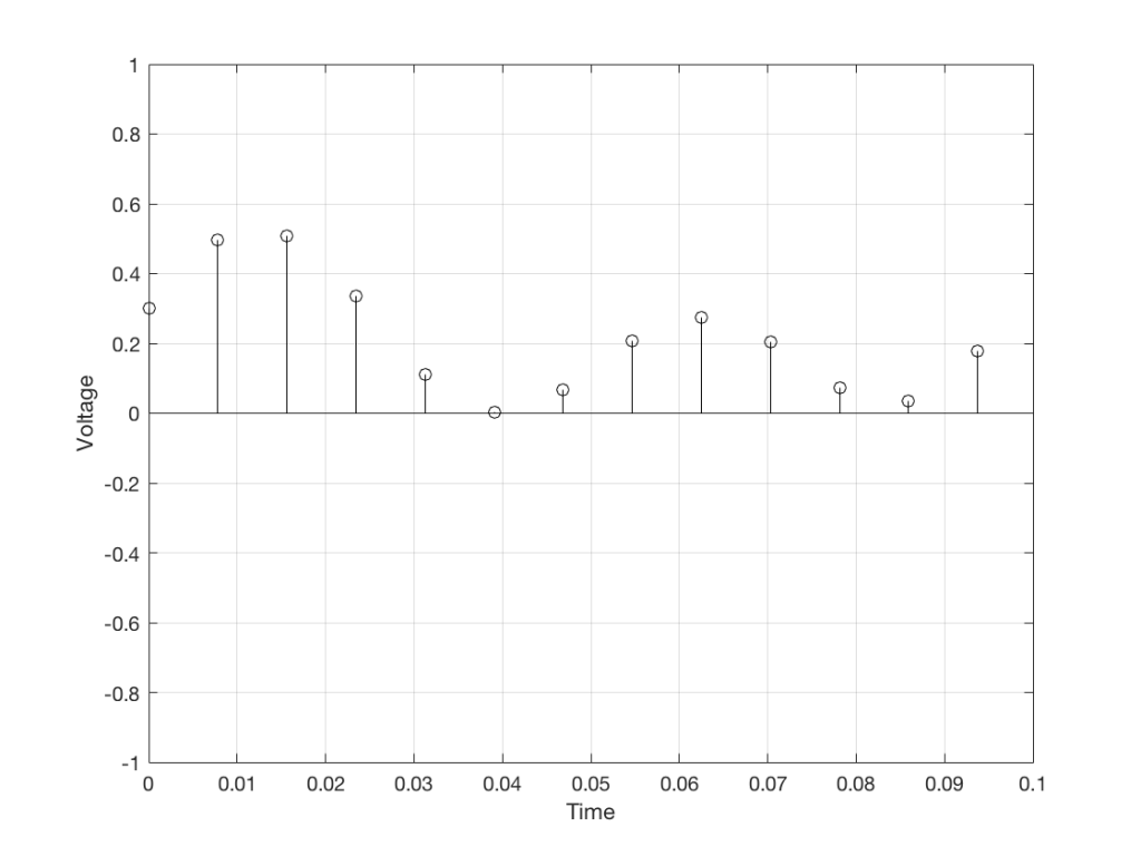
We can then keep the measurements (remembering how often we made them…) and write them down like this:
0.3000
0.4950
0.5089
0.3351
0.1116
0.0043
0.0678
0.2081
0.2754
0.2042
0.0730
0.0345
0.1775
We can store this series of numbers on a computer’s hard disk, for example. We can then come back tomorrow, and convert the measurements to voltages. First we read the measurements, and create the appropriate voltage…
We then make a “staircase” waveform by “holding” those voltages until the next value comes in.
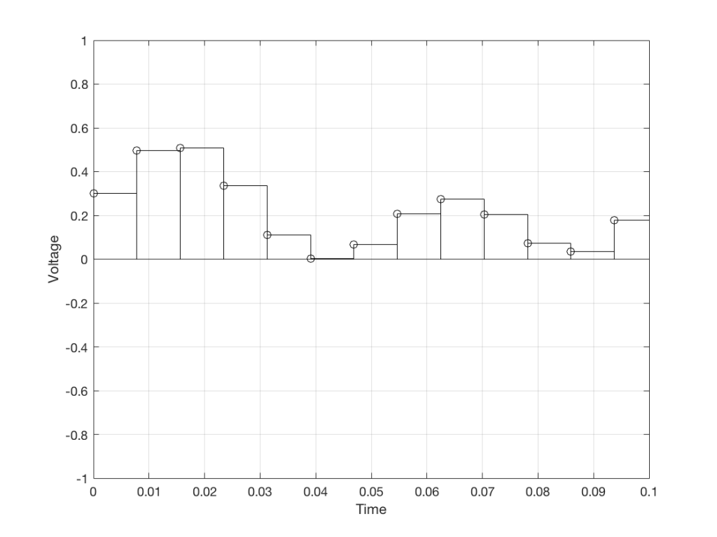
All we need to do then is to use a low-pass filter to smooth out the hard edges of the staircase.
So, in this example, we’ve gone from an analogue signal (the red curve in Figure 3) to a digital signal (the series of numbers), and back to an analogue signal (the red curve in Figure 7).
In some ways, this is a bit like the way a movie works. When you watch a movie, you see a series of still photographs, probably taken at a rate of 24 pictures (or frames) per second. If you play those photos back at the same rate (24 fps or frames per second), you think you see movement. However, this is because your eyes and brain aren’t fast enough to see 24 individual photos per second – so you are fooled into thinking that things on the screen are moving.
However, digital audio is slightly different from film in two ways:
- The sound (equivalent to the movement in the film) is actually happening. It’s not a trick that relies on your ears and brain being too slow.
- If, when you were filming the movie, something were to happen between frames (say, the flash of a gunshot, for example) then it would never be caught on film. This is because the photos are discrete moments in time – and what happens between them is lost. However, if something were to make a very, very short sound between two samples (two measurements) in the digital audio signal – it would not be lost. This is because of something that happens at the beginning of the chain that I haven’t described… yet…
However, there are some “artefacts” (a fancy term for “weird errors”) that are present both in film and in digital audio that we should talk about.
The first is an error that happens when you mess around with the rate at which you take the measurements (called the “sampling rate”) or the photos (called the “frame rate”) – and, more importantly, when you need to worry about this. Let’s say that you make a film at 24 fps. If you play this back at a higher frame rate, then things will move very quickly (like old-fashioned baseball movies…). If you play them back at a lower frame rate, then things move in slow motion. So, for things to look “normal” you have to play the movie at the same rate that it was filmed. However, as longs no one is looking, you can transfer the movie as fast as you like. For example, if you wanted to copy the film, you could set up a movie camera so it was pointing at a movie screen and film the film. As long as the movie on the screen is running in sync with the camera, you can do this at any frame rate you like. But you’ll have to watch the copy at the same frame rate as the original film…
The second is an easy artefact to recognise. If you see a car accelerating from 0 to something fast on film, you’ll see the wheels of the car start to get faster and faster, then, as the car gets faster, the wheels slow down, stop, and then start going backwards… This does not happen in real life (unless you’re in a place lit with flashing lights like fluorescent bulbs or LED’s). I’ll do a posting explaining why this happens – but the thing to remember here is that the speed of the wheel rotation that you see on the film (the one that’s actually captured by the filming…) is not the real rotational speed of the wheel. However, those two rotational speeds are related to each other (and to the frame rate of the film). If you change the real rotational rate or the frame rate, you’ll change the rotational rate in the film. So, we call this effect “aliasing” because it’s a false version (an alias) of the real thing – but it’s always the same alias (assuming you repeat the conditions…) Digital audio can also suffer from aliasing, but in this case, you put in one frequency (which is actually the same as a rotational speed) and you get out another one. This is not the same as harmonic distortion, since the frequency that you get out is due to a relationship between the original frequency and the sampling rate, so the result is almost never a multiple of the input frequency.
Some details that I left out…
One of the things I said above was something like “we measure the voltage and store the results” and the example I gave was a nice series of numbers that only had 4 digits after the decimal point. This statement has some implications that we need to discuss.
Let’s say that I have a thing that I need to measure. For example, Figure 8 shows a piece of metal, and I want to measure its width.
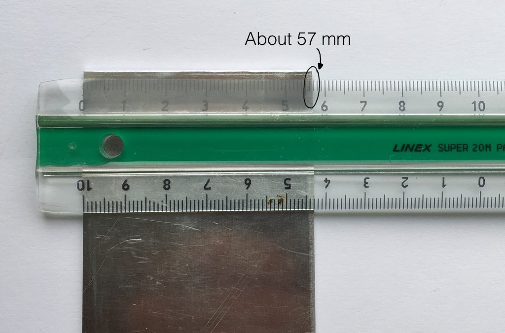
Using my ruler, I can see that this piece of metal is about 57 mm wide. However, if I were geeky (and I am) I would say that this is not precise enough – and therefore it’s not accurate. The problem is that my ruler is only graduated in millimetres. So, if I try to measure anything that is not exactly an integer number of mm long, I’ll either have to guess (and be wrong) or round the measurement to the nearest millimetre (and be wrong).
So, if I wanted you to make a piece of metal the same width as my piece of metal, and I used the ruler in Figure 8, we would probably wind up with metal pieces of two different widths. In order to make this better, we need a better ruler – like the one in Figure 9.
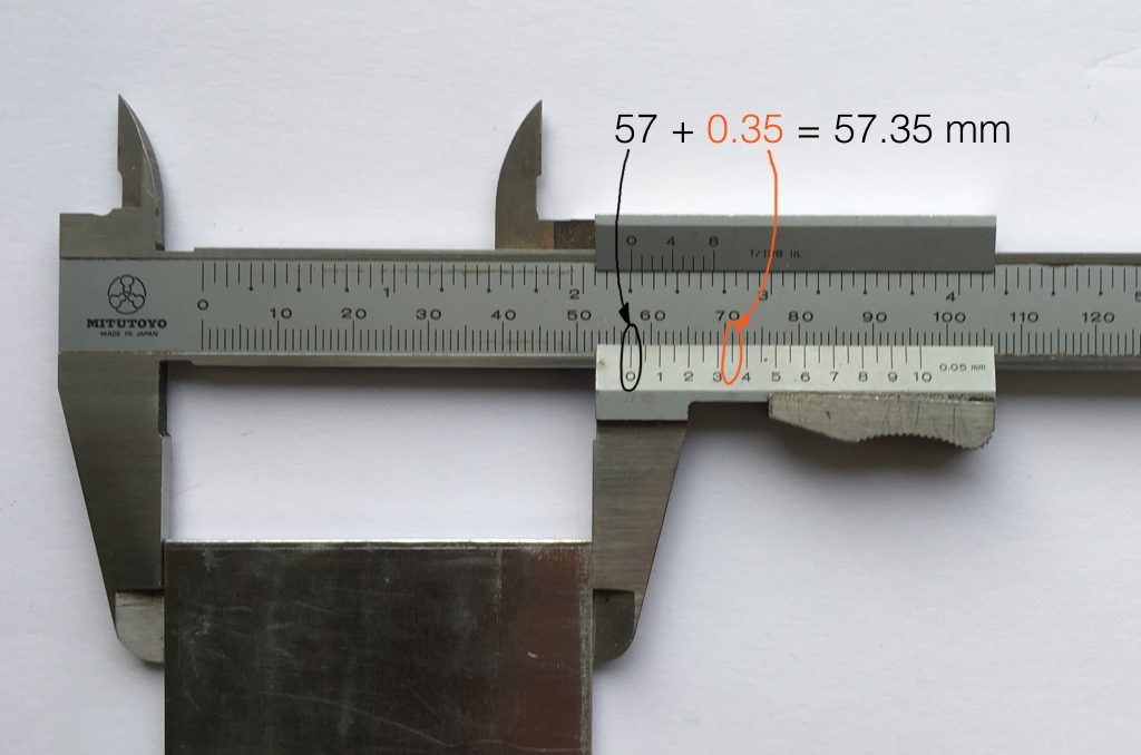
Figure 9 shows a vernier caliper (a fancy type of ruler) being used to measure the same piece of metal. The caliper has a resolution of 0.05 mm instead of the 1 mm available on the ruler in Figure 8. So, we can make a much more accurate measurement of the metal because we have a measuring device with a higher precision.
The conversion of a digital audio signal is the same. As I said above, we measure the voltage of the electrical signal, and transmit (or store) the measurement. The question is: how accurate and precise is your measurement? As we saw above, this is (partly) determined by how many digits are in the number that you use when you “write down” the measurement.
Since the voltage measurements in digital audio are recorded in binary rather than decimal (we use 0 and 1 to write down the number instead of 0 up to 9) then we use Binary digITS – or “bits” instead of decimal digits (which are not called “dits”). The number of bits we have in the number that we write down (partly) determines the precision of the measurement of the voltage – and therefore (possibly), our accuracy…
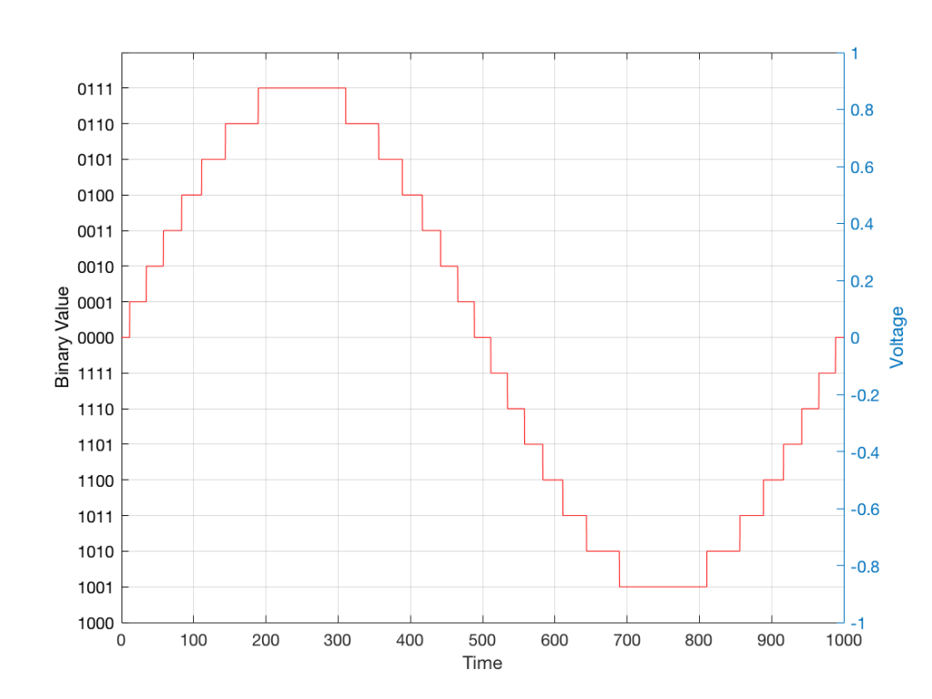
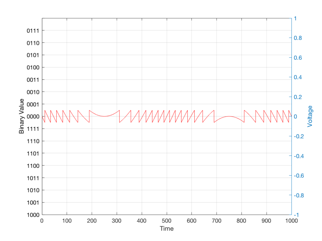
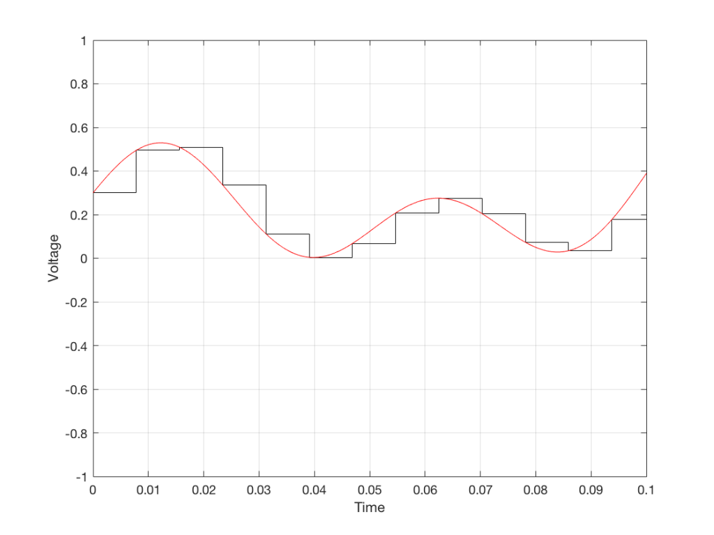
Just like the example of the ruler in Figure 8, above, we have a limited resolution in our measurement. For example, if we had only 4 bits to work with then the waveform in 4 – the one we have to measure – would be measured with the “ruler” shown on the left side of Figure 10, below.
When we do this, we have to round off the value to the nearest “tick” on our ruler, as shown in Figure 11.
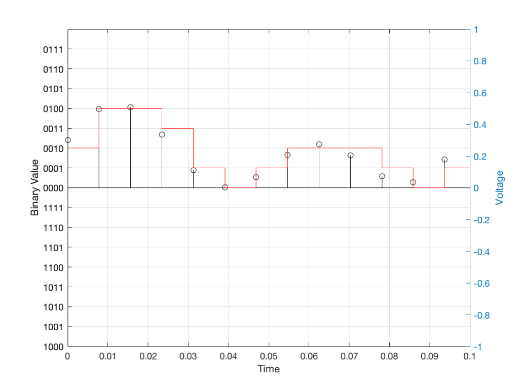
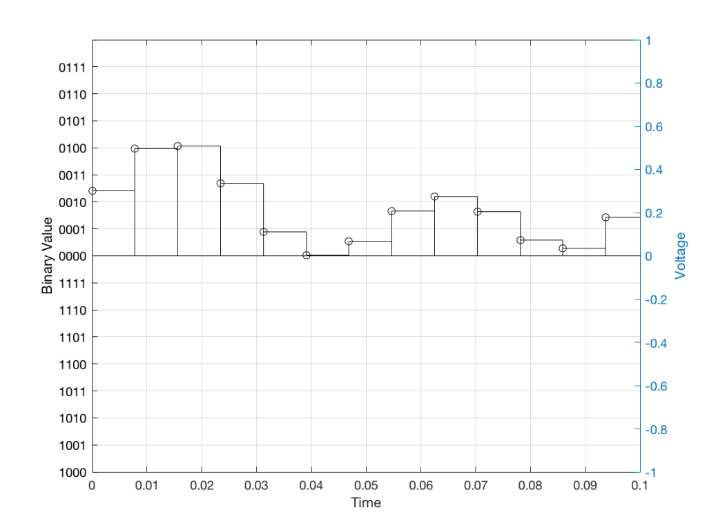
Using this “ruler” which gives a write-down-able “quantity” to the measurement, we get the following values for the red staircase:
0010
0100
0100
0011
0001
0000
0001
0010
0010
0010
0001
0000
0001
When we “play these back” we get the staircase again, shown in Figure 12.
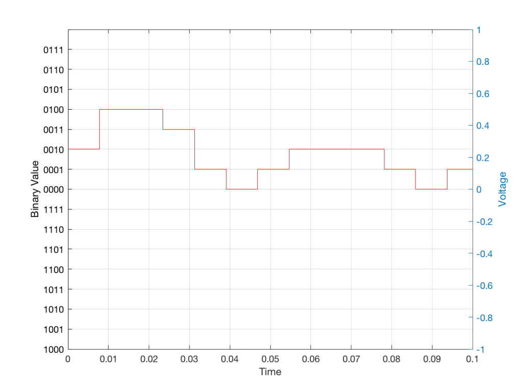
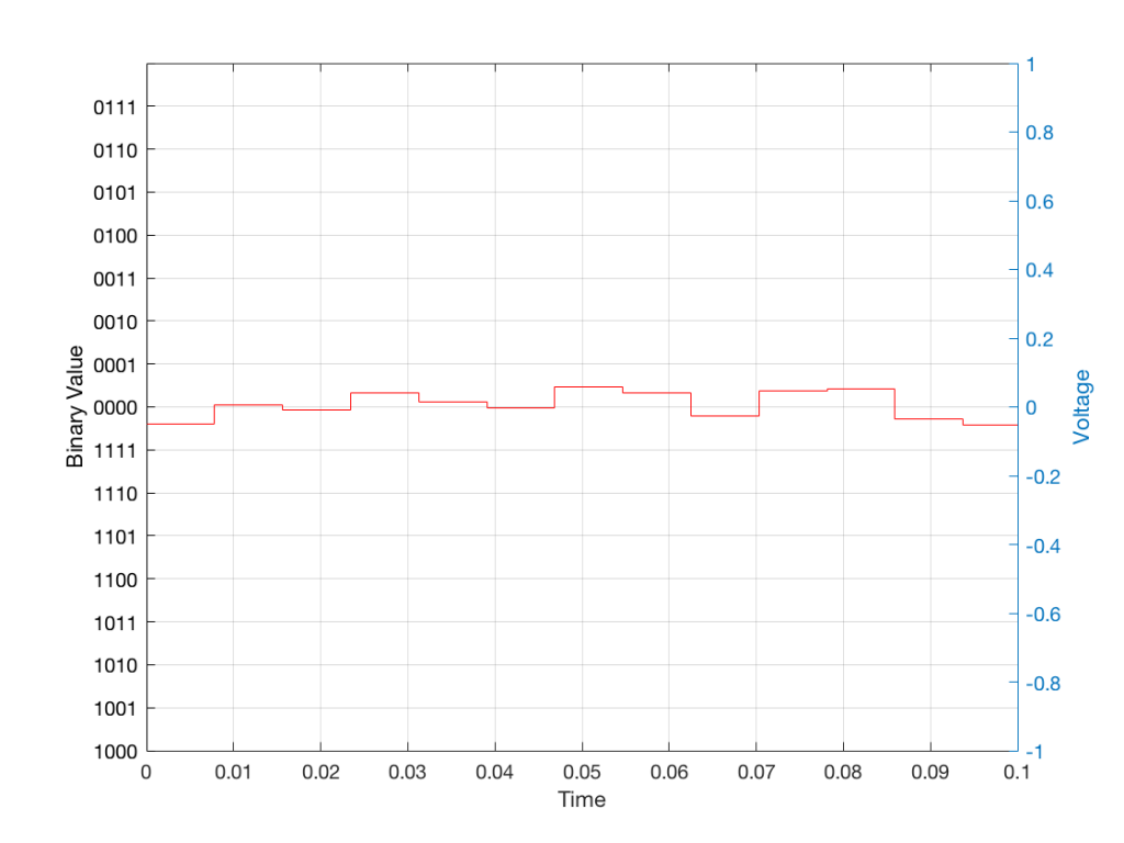
Of course, this means that, by rounding off the values, we have introduced an error in the system (just like the measurement in Figure 8 has a bigger error than the one in Figure 9). We can calculate this error if we just subtract the original signal from the output signal (in other words, Figure 12 minus Figure 10) to get Figure 13.
In order to improve our accuracy of the measurement, we have to increase the precision of the values. We can do this by adding an extra digit (or bit) to the number that we use to record the value.
If we were using decimal numbers (0-9) then adding an extra digit to the number would give us 10 times as many possibilities. (For example, if we were using 4 digits after the decimal in the example at the start of this posting, we have a total of 10,000 possible values – 0.0000 to 0.9999. If we add one more digit, we increase the resolution to 100,000 possible values – 0.00000 to 0.99999 ).
In binary, adding one extra digit gives us twice as many “ticks” on the ruler. So, using 4 bits gives us 16 possible values. Increasing to 5 bits gives us 32 possible values.
If you’re listening to a CD, then the individual measurements of each voltage – the “sample values” – are stored with 16 bits, which means that we have 65,536 possible values to pick from.
Remember that this means that we have more “ticks” on our ruler – but we don’t necessarily increase its range. So, for example, we’re still measuring a voltage from -1 V to 1 V – we just have more and more resolution to do that measurement with.
Error #1
Finally! We get to the beginning of the point of the posting in the first place. My whole reason for starting this series of postings was to talk about errors in digital audio.
So, the first one to talk about is whether we have “bit matching” in a system where we expect to do so. For example, if you look at the S/P-DIF output of a good-old-fashioned CD player, do the sample values that are transmitted on that wire identical to the ones on the disc?
This is a fairly easy test to make (in theory). All you have to do is to record the digital signal on the S/P-DIF output of your CD player, subtract the original signal that’s on the disc (making sure that you have done your time alignment correctly). If you have anything other than nothing left over, then something went wrong somewhere.
If the result of this test is that you do NOT get nothing remaining, you cannot jump in head first and say that your S/P-DIF output is not working properly. For example, some sound cards have a sampling rate converter at their digital input. So, if you are capturing the CD player’s output using such a sound card on your computer, then perhaps the errors that you see are being produced by your sound card – and not your player.
A little associated story
This was a method that I used to do the final testing of Wireless Power Link for B&O. I created a little software application that made a signal and sent it out digitally to a Wireless Power Link transmitter (which was running with a resolution of 24 bits – giving us 16,777,216 possible values). I then connected a Wireless Power Link receiver’s output to the same computer. The computer knew how much time it took the signal to get from its output, through the wireless transmission system, back to its input (about 5 ms). So, I took the “output” signal, delayed it by that amount, and then subtracted it from the “input” signal. I then made a detector that counted every bit (instead of every sample) that was incorrect.
The reason I was counting bit errors instead of sample errors was that we wanted to be able to diagnose problems if we found them. If you find out that “this sample is wrong” – you don’t necessarily know whether it was one or more bit errors that caused the problem. By counting bit errors, you have a little more information that can help you diagnose the source of problems when you find them.
Sidebar: since this test was running at 48 kHz and 24 bits with a 2-channel system, that means that there were 2,304,000 bits per second being checked every second
This test ran 24-hours a day continuously for over 11 days. In that time, we found 0 bit errors. That means that we got 0 errors in more than 2,189,721,600,000 bits, which was good.
Now, just before anyone gets excited: that test was run to find out whether the WPL system was able to deliver a bit-perfect output in the absence of any external disturbances. So, the transmitter and the receiver were not moved at any time during the test, and nothing was moved between them – and the result was that the system behaved perfectly.
B&O Tech: BeoLab loudspeakers and Third-party systems
#77 in a series of articles about the technology behind Bang & Olufsen loudspeakers
I’m occasionally asked about the technical details of connecting Bang & Olufsen loudspeakers to third-party (non-B&O) sources. In the “old days”, this was slightly difficult due to connectors, adapters, and outputs. However, that was a long time ago – although beliefs often persist longer than facts…
All Bang & Olufsen “BeoLab” loudspeakers are “active”. At the simplest level, this means that the amplifiers are built-in. In addition, almost all of the BeoLab loudspeakers in the current portfolio use digital signal processing. This means that the filtering and crossovers are implemented using a built-in computer instead of using resistors, capacitors, and inductors. This will be a little important later in this posting.
In order to talk about the compatibility issues surrounding the loudspeakers in the BeoLab portfolio – both with themselves and with other loudspeakers, we really need to break the discussion into two areas. The first is that of connectors and signals. The second, more problematic issue is that of “latency” (which is explained below…)
Connectors and signals
Since BeoLab loudspeakers have the amplifiers built-in, you need to connect them to an analogue “line level” signal instead of the output of an amplifier.
This means that, if you have a stereo preamplifier, then you just connect the “volume-regulated” Line Output of the preamp to the RCA line inputs of the BeoLab loudspeakers. (Note that the BeoLab 3 does not have a built-in RCA connector, so you need an adapter for this). Since the BeoLab loudspeakers (except for BeoLab 5, 50, and 90) are fixed at “full volume”, then you need to ensure that your Line Output of the source is, indeed, volume-regulated. If not, things will be surprisingly loud…
In addition to the RCA Line inputs, most BeoLab loudspeakers also have at least one digital audio input. The BeoLab 5 has an S/P-DIF “coaxial” input. The BeoLab 17, 18, and 20 have optical digital inputs. The BeoLab 50 and 90 have many options to choose from. Again, apart from the BeoLab 5, 50, and 90, the loudspeakers are fixed at “full volume”, so if you are going to use the digital input for the BeoLab 17, 18, or 20, you will need to enable the volume regulation of the digital output of your source, if that’s possible.
Latency
Any audio device has some inherent “latency” or “delay from the time the signal comes in until it goes out”. For some devices, this latency can be so low that we can think of it as being 0 seconds. In other words, for some devices (say, a wire, for example) the signal comes out at the same time as it comes in (as far as we’re concerned… I’m not going to get into an argument about the speed of electricity or light, since these go very fast…)
Any audio device that uses digital signal processing has some measurable (and possibly audible) latency. This is primarily due to 5 things, seen in the flowchart below.
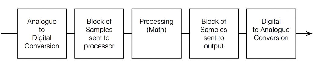
Each of these 5 steps each have different amounts of latency – some of them very, very small. Some are bigger. One thing to know about digital signal processing is that, typically, in order to make the math more efficient (and therefore squeeze as much as possible out of the computing power), the samples are processed in “blocks” – not one-by-one. So, the signal comes into the input, it gets converted to individual samples, and those samples are collected into a block of 64 samples (for example) before being sent to the processing.
So, let’s say that you have a sampling rate of 44100 samples per second, and a block size of 64 samples. This then means that you send a block to the processor every 64 * 1/44100 = 1.45 ms. That block gets processed (which takes some time), and then sent as another block of 64 samples to the DAC (digital to analogue converter).
So, ignoring the latency of the conversion from- and to-analogue, in the example above, it will take 1.45 ms to get the signal into the processor, you have a 1.45 time window to do the processing, and it will take another 1.45 ms to get the signal out to the DAC. This is a total of 4.35 ms from the instant a signal gets comes into the analogue input to the moment it comes out the analogue output.
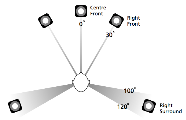
Sidebar: Of course, 4.3 ms is not a long time. If you had a loudspeaker outdoors, then adding 4.35 ms to its latency would be same delay you would incur by moving 1.5 m (or about 4.9 feet) further away. However, in terms of a stereo or multichannel audio system, 4.35 ms is an eternity. For example, if you have a correctly-configured stereo loudspeakers (with each loudspeaker 30º from centre-front, and you’re sitting in the “sweet spot”, if you delay the left loudspeaker by just 0.2 ms, then lead vocals in your pop tunes will move 10º to the right instead of being in the centre. It only takes 1.12 ms of delay in one loudspeaker to move things all the way to the opposite side. In a multichannel loudspeaker configuration (or in headphones), some of the loudspeaker pairs (e.g. Left Surround – Right Surround) result in you being even more sensitive to these so-called “inter-channel delay differences”.
Also, the amount of time required by the processing depends on what kind of processing you’re doing. In the case of BeoLab 50 and 90, for example, we are using FIR filters as part of the directivity (Beam Width and Beam Direction) processing. Since this filtering extends quite low in frequency, the FIR filters are quite long – and therefore they require extra latency. To add a small amount of confusion to this discussion (as we’ll see below) this latency is switchable to be either 25 ms or 100 ms. If you want Beam Width control to extend as low in frequency as possible, you need to use the 100 ms “Long Latency” mode. However, if you need lip-synch with a non-B&O source, you should use the 25 ms “Low Latency” mode (with the consequent loss of directivity control at very low frequencies).
Latency in BeoLab loudspeakers
In order to use BeoLab loudspeakers with a non-B&O source (or an older B&O source) , you may need to know (and compensate for) the latency of the loudspeakers in your system. This is particularly true if you are “mixing and matching” loudspeakers: for example, using different loudspeaker models (or other brands – *gasp*) in a single multichannel configuration.
| Model | A / D | Latency (ms) | Equivalent in m | Volume Regulation? |
| Unknown analogue | A | 0 | 0 | No |
| Beolab 1 | A | 0 | 0 | No |
| Beolab 2 | A | 0 | 0 | No |
| Beolab 3 | A | 0 | 0 | No |
| Beolab 4 | A | 0 | 0 | No |
| Beolab 5 | D | 3.92 | 1.35 | Yes |
| Beolab 7 series | A | 0 | 0 | No |
| Beolab 9 | A | 0 | 0 | No |
| Beolab 12 series | D | 4.4 | 1.51 | No |
| Beolab 17 | D | 4.4 | 1.51 | No |
| Beolab 18 | D | 4.4 | 1.51 | No |
| Beolab 19 | D | 4.4 | 1.51 | No |
| Beolab 20 | D | 4.4 | 1.51 | No |
| Beolab 50 | D | 25 / 100 | 8.6 / 34.4 | Yes |
| Beolab 90 | D | 29 / 100 | 10.0 / 34.4 | Yes |
How to Do It
I’m going to make two assumptions for the rest of this posting:
- you have a stereo preamp or a surround processor / AVR that has a “Speaker Distance” or “Speaker Delay” adjustment parameter (measured from the loudspeaker location to the listening position)
- it does not have a “loudspeaker latency” adjustment parameter
The simple version (that probably won’t work):
Since the latency of the various loudspeakers can be “translated” into a distance, and since AVR’s typically have a “Speaker Distance” parameter, you simply have to add the equivalent distance of the loudspeaker’s latency to the actual distance to the loudspeaker when you enter it in the menus.
For example, let’s say that you have a 5.0 channel loudspeaker configuration with the following actual speaker distances, measured in the room.
| Channel | Model | Distance |
| Left Front | Beolab 5 | 3.7 |
| Right Front | Beolab 5 | 3.9 |
| Centre Front | Beolab 3 | 3.9 |
| Left Surround | Beolab 17 | 1.6 |
| Right Surround | Beolab 17 | 3.2 |
You then look up the equivalent distances in the first table and add the appropriate number to each loudspeaker.
| Channel | Model | Distance | + | Latency Equivalent | = | Total |
| Left Front | Beolab 5 | 3.7 | + | 1.35 | = | 5.05 |
| Right Front | Beolab 5 | 3.9 | + | 1.35 | = | 5.25 |
| Centre Front | Beolab 3 | 3.9 | + | 0 | = | 3.9 |
| Left Surround | Beolab 17 | 1.6 | + | 1.51 | = | 3.11 |
| Right Surround | Beolab 17 | 3.2 | + | 1.51 | = | 4.71 |
This technique will work fine unless the total distance that you have to enter in the AVR’s menus is greater than its maximum possible value (which is typically 10.0 m on most brands and models that I’ve seen – although there are exceptions).
So, what do you do if your AVR can’t handle a value that’s high enough? Then you need to fiddle with the numbers a bit…
The slightly-more complicated version (which might work most of the time)
When you enter the Speaker Distances in the menus of your AVR, you’re doing two things:
- calibrating the delay compensation for the differences in the distances from the listening position to the individual loudspeakers
- (maybe) calibrating the system to ensure that the sound arrives at the listening position at the same time as the video is displayed on the screen (therefore sending the sound out early, since it takes longer for the sound to travel to the sofa than it takes the light to get from your screen…)
That second one has a “maybe” in front of it for a couple of reasons:
- this is a very small effect, and might have been decided by the manufacturer to be not worth the effort
- the manufacturer of an AVR has no way of knowing the latency of the screen to which it’s attached. So, it’s possible that, by outputting the sound earlier (to compensate for the propagation delay of the sound) it’s actually making things worse (because the screen is delayed, but the AVR doesn’t know it…)
So, let’s forget about that lip-synch issue and stick with the “delay compensation for the differences in the distances” issue. Notice that I have now highlighted the word “differences” in italics twice… this is important.
The big reason for entering Speaker Distances is that you want the a sound that comes out of all loudspeakers simultaneously to reach the listening position simultaneously. This means that the closer loudspeakers have to wait for the further loudspeakers (by adding an appropriate delay to their signal path). However, if we ignore the synchronisation to another signal (specifically, the lips on the screen), then we don’t need to know the actual (or “absolute”) distance to the loudspeakers – we only need to know their differences (or “relative distances”). This means that you can consider the closest loudspeaker to have a distance of 0 m from the listening position, and you can subtract that distance from the other distances.
For example, using the table above, we could subtract the distance to the closest loudspeaker (the Left Surround loudspeaker, with a distance of 1.6 m) from all of the loudspeakers in the table, resulting in the table below.
| Channel | Model | Distance | – | Closest | = | Result |
| Left Front | Beolab 5 | 3.7 | – | 1.6 | = | 2.1 |
| Right Front | Beolab 5 | 3.9 | – | 1.6 | = | 2.3 |
| Centre Front | Beolab 3 | 3.9 | – | 1.6 | = | 2.3 |
| Left Surround | Beolab 17 | 1.6 | – | 1.6 | = | 0 |
| Right Surround | Beolab 17 | 3.2 | – | 1.6 | = | 1.6 |
Again, you look up the equivalent distances in the first table and add the appropriate number to each loudspeaker.
| Channel | Model | Distance | + | Latency equivalent | = | Total |
| Left Front | Beolab 5 | 2.1 | + | 1.35 | = | 3.45 |
| Right Front | Beolab 5 | 2.3 | + | 1.35 | = | 3.65 |
| Centre Front | Beolab 3 | 2.3 | + | 0 | = | 2.3 |
| Left Surround | Beolab 17 | 0 | + | 1.51 | = | 1.51 |
| Right Surround | Beolab 17 | 1.6 | + | 1.51 | = | 3.11 |
As you can see in Table 5, the end results are smaller than those in Table 3 – which will help if your AVR can’t get to a high enough value for the Speaker Distance.
The only-slightly-even-more complicated version (which has a better chance of working most of the time)
Of course, the version I just described above only subtracted the smallest distance from the other distances, however, we could do this slightly differently and subtract the smallest total (actual + equivalent distance) from the totals to “force” one of the values to 0 m. This can be done as follows:
Starting with a copy of Table 3, we get a preliminary Total, and then subtract the smallest of these from all value to get our Final Speaker Distance.
| Channel | Model | Distance (m) | + | Latency (m) | = | Total | – | Smallest | = | Final |
| Lf | BL 5 | 3.7 | + | 1.35 | = | 5.05 | – | 3.11 | = | 1.94 |
| Rf | BL 5 | 3.9 | + | 1.35 | = | 5.25 | – | 3.11 | = | 2.14 |
| Cf | BL 3 | 3.9 | + | 0 | = | 3.9 | – | 3.11 | = | 0.79 |
| Ls | BL17 | 1.6 | + | 1.51 | = | 3.11 | – | 3.11 | = | 0 |
| Rs | BL 17 | 3.2 | + | 1.51 | = | 4.71 | – | 3.11 | = | 1.6 |
Of course, if you do it the first way (as shown in Table 3) and the values are within the limits of your AVR, then you don’t need to get complicated and start subtracting. And, in many cases, if you don’t own BeoLab 50 or 90, and you don’t live in a mansion, then this will probably be okay. However… if you DO own BeoLab 50 or 90, and/or you do live in a mansion, then you should probably get used to subtracting…
Some additional information about BeoLab 50 & 90
As I mentioned above, the BeoLab 50 and BeoLab 90 have two latency options. The “High Latency” option (100 ms) allows us to implement FIR filters that control the directivity (the Beam Width and Beam Directivity) to as low a frequency as possible. However, in this mode, the latency is so high that you will notice that the sound is behind the picture if you have a non-B&O television.* In other words, you will not have “lip-synch”.
For customers with a non-B&O television*, we have included a “Low Latency” option (25 ms) which is within the tolerable limits of lip-synch. In this mode, we are still controlling the directivity of the loudspeaker with an FIR, but it cannot go as low in frequency as the “High Latency” option.
As I mentioned above, a 100 ms latency in a loudspeaker is equivalent to placing it 34.4 m further away (ignoring the obvious implications on the speaker level). If you have a third-part source such as an AVR, it is highly unlikely that you can set a Speaker Distance in the menus to be the actual distance + 34.4 m…
So, in the case of BeoLab 50 or 90, you should manually set the Latency Mode to “Low Latency” (using the setup options in the speaker’s app). This then means that you should add “only” 8.6 m to the actual distance to the loudspeaker.
Of course, if you are using the BeoLab 50 or 90 alone (meaning that there is no video signal, and no other loudspeakers that need time-alignment) then this is irrelevant, and you can just set the Speaker Distance to 0 m. You can also change the loudspeakers to another preset (that you or your installer set up) that uses the High Latency mode for best performance.
Instructions on how to do this are found in the Technical Sound Guide for the BeoLab 50 or the BeoLab 90 via the Bang & Olufsen website at www.bang-olufsen.com.
* Here a “B&O Television” means a BeoPlay V1, BeoVision 11, 14, Avant, Avant NG, Horizon, or Eclipse. Older B&O televisions are different… This will be discussed in the next blog posting.
Modern acoustical design

B&O Tech: Distance Tweaking
#75 in a series of articles about the technology behind Bang & Olufsen loudspeakers
So, you’ve just installed a pair of loudspeakers, or a multichannel surround system. If you’re a normal person then you have not set up your system following the recommendations stated in the International Telecommunications Union’s document “Rec. ITU-R BS.775-1: MULTICHANNEL STEREOPHONIC SOUND SYSTEM WITH AND WITHOUT ACCOMPANYING PICTURE”. That document states that, in a best case, you should use a loudspeaker placement as is shown below in Figure 1.
In a typical configuration, the loudspeakers are NOT the same distance from the listening position – and this is a BIG problem if you’re worried about the accuracy of phantom image placement. Why is this? Well, let’s back up a little…
Localisation in the Real World
Let’s say that you and I were standing out in the middle of a snow-covered frozen pond on a quiet winter day. I stand some distance away from you and we have a conversation. When I’m doing the talking, the sound of my voice leaves my mouth and moves towards you.
If I’m directly in front of you, then the sound (in theory) arrives at both of your ears simultaneously (resulting in an Interaural Time Difference or ITD of 0 ms) and at exactly the same level (resulting in an Interaural Amplitude Difference or IAD of 0 dB). Your brain detects that the ITD is 0 ms and the IAD is 0 dB, and decides that I must be directly in front of you (or directly behind you, or above you – at least I must be somewhere on your sagittal plane…)
If I move slightly to your left, then two things happen, generally speaking. Firstly, the sound of my voice arrives at your left ear before your right ear because it’s closer to me. Secondly, the sound of my voice is generally louder in your left ear than in your right ear, not only because it’s closer, but (mostly) because your head shadows your right ear from the sound of my voice. So, you brain detects that my voice is earlier and louder in your left ear, so I must be somewhere on your left.
Of course, there are many other, smaller cues that tell you where the sound is coming from exactly – but we don’t need to get into those details today.
There are two important thing to note here. The first is that these two principal cues – the ITD and the IAD – are not equally important. If they got in a fight, the ITD would win. If a sound arrived at your left ear earlier, but was louder in your right ear, it would have to be a LOT louder in the right ear to convince you that you should ignore the ITD information…
The second thing is that the time differences we’re talking about are very very small. If I were directly to one side of you, looking directly at your left ear, say… then the sound would arrive at your right ear approximately only 700 µs – that’s 700 millionths of a second or 0.0007 seconds later than at your left ear.
So, the moral of this story so far is that we are very sensitive to differences in the time of arrival of a sound at our two ears.
Localisation in a reproduced world
Now go back to the same snow-covered frozen lake with a pair of loudspeakers instead of bringing me along, and set them up in a standard stereo configuration, where the listening position and the two loudspeakers form an equilateral triangle. This means that when you sit and listen to the signals coming out of the loudspeakers
- the two loudspeakers are the same distance from the listening position, and
- the left loudspeaker is 30º to the left of front-centre, and the right loudspeaker is 30º to the right of front-centre.
Have a seat and we’ll play some sound. To start, we’ll play the same sound in both loudspeakers at exactly the same time, and at exactly the same level. Initially, the sound from the left loudspeaker will reach your left ear, and the sound from the right loudspeaker reaches your right ear. A very short time later the sound from the left loudspeaker reaches your right ear and the sound from the right loudspeaker reaches your left ear (this effect is called Interaural Crosstalk – but that’s not important). After this, nothing happens, because you are sitting in the middle of a frozen lake covered in snow – so there are no reflections from anything.
Since the sounds in the two loudspeakers are identical, then the sounds in your ears are also identical to each other. And, just as is the case in real-life, if the sounds in your two ears are identical, you’ll localise the sound source as coming from somewhere on your sagittal plane. Due to some other details in the localisation cues that we’re not talking about here, chances are that you’ll hear the sound as originating from a position directly in front of you – between the two loudspeakers.
Because the apparent location of that sound is a position where there is no loudspeaker, it’e like a ghost – so it’s called a “phantom centre” image.
That’s the centre image, but how do we move the image slightly to one side or the other? It’s actually really easy – we just need to remember the effects of ITD and IAD, and do something similar.
So, if I play a sound out of both loudspeakers at exactly the same time, but I make one loudspeaker slightly louder than the other, then the phantom image will appear to come from a position that is closer to the louder loudspeaker. So, if the right channel is louder than the left channel, then the image appears to come from somewhere on the right. Eventually, if the right loudspeaker is louder enough (about 15 dB, give or take), then the image will appear to be in that loudspeaker.
Similarly, if I were to keep the levels of the two loudspeakers identical, but I were to play the sound out of the right loudspeaker a little earlier instead, then the phantom image will also move towards the earlier loudspeaker.
There have been many studies done to find out exactly what apparent phantom image position results from exactly what level or delay difference between the two loudspeakers (or a combination of the two). One of the first ones was done by Gert Simonsen in 1983, in which he found the following results.
[table]
Image Position, Amplitude difference, Time difference
0º, 0.0 dB, 0.0 ms
10º, 2.5 dB, 0.2 ms
20º, 5.5 dB, 0.44 ms
30º, 15.0 dB, 1.12 ms
[/table]
Note that this test was done with loudspeakers at ±30º – so the bottom line of the table means “in one of the loudspeakers”. Also, I have to be clear that the values in this table are NOT to be used concurrently. So, this shows the values that are needed to produce the desired phantom image location using EITHER amplitude differences OR time differences.
Again, the same two important points apply.
Firstly, the time differences are a more “powerful” cue than the amplitude differences. In other words, if the left loudspeaker is earlier, but the right loudspeaker is louder, you’ll hear the phantom image location towards the left, unless the right loudspeaker is a LOT louder.
Secondly, you are VERY sensitive to time differences. The left loudspeaker only needs to be 1.12 ms earlier than the right loudspeaker in order for the phantom image to move all the way into that loudspeaker. That’s equivalent to the left loudspeaker being about 38.5 cm closer than the right loudspeaker (because the speed of sound is about 344 m/s (depending on the temperature) and 0.00112 * 344 = 0.385 m).
Those last two paragraphs were the “punch line” – if the distances to the loudspeakers are NOT the same, then, unless you do something about it, you’ll wind up hearing your phantom images pulling towards the closer loudspeaker. And it doesn’t take much of an error in distance to produce a big effect.
Whaddya gonna do about it?
Almost every surround processor and Audio Video Receiver in the world gives you the option of entering the Speaker Distances in a menu somewhere. There are two possible reasons for this.
The first is not so important – it’s to align the sound at the listening position with the video. If you’re sitting 3 m from the loudspeakers and the TV, then the sound arrives 8.7 ms after you see the picture (the same is true if you are listening to a person speaking 3 m away from you). To eliminate this delay, the loudspeakers could produce the sound 8.7 ms too early, and the sound would reach you at the same time as you see the video. As I said, however, this is not a problem to lose much sleep over, unless you sit VERY far away from your television.
The second reason is very important, as we’ve already seen. If, as we established at the start of this posting, you’re a normal person, then your loudspeakers are not all the same distance from the listening position. This means that you should apply a delay to the closer loudspeaker(s) to get them to “wait” for the sound as it travels towards you from the further loudspeakers. That way, if you have the same sound in all channels at the same time, then the loudspeaker do NOT produce it at the same time, but it arrives at the listening position simultaneously, as it should.
Problem solved! Right?
Wrong.
Corrections that need correcting
Let’s make a configuration of a pair of loudspeakers and a listening position that is obviously wrong.
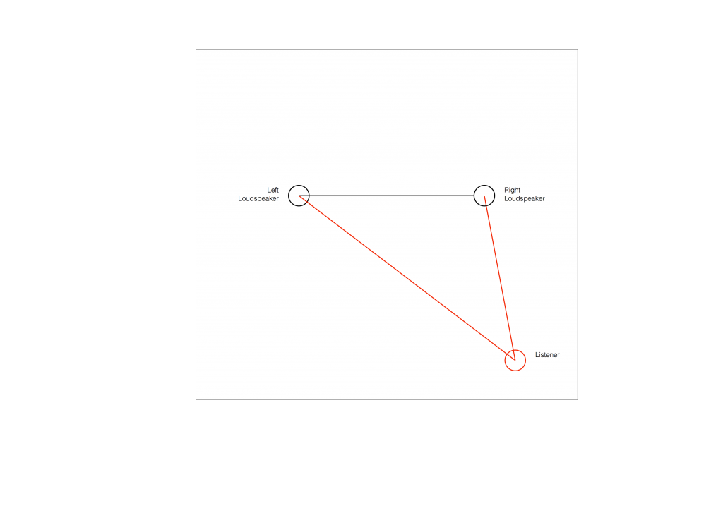
Figure 2 shows the example of a very bad loudspeaker configuration for stereo listening. (I’m keeping things restricted to two channels to keep things simple – but multichannel is the same…) The right loudspeaker is much closer than the left loudspeaker, so all phantom images will appear to “bunch together” into the right loudspeaker.
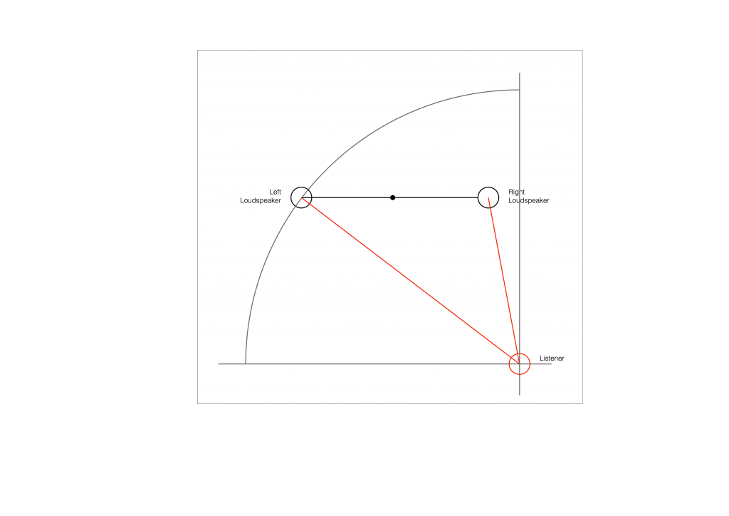
So, to do the correction, you measure the distances to the two loudspeakers from the listening position and enter those two values into the surround processor. It then subtracts the smaller distance from the larger distance, converts that to a delay time, and delays the closer loudspeaker by that amount to compensate for the difference.

So, after the delay is applied to the closer loudspeaker, in theory, you have a stereo pair of loudspeakers that are equidistant from the listening position. This means that, instead of hearing (for example) the phantom centre images in the closer loudspeaker, you’ll hear it as being positioned at the centre point between the distant loudspeaker (the left one, in this example) and the “virtual” one (the right one in this example). This is shown below.

As you can see in Figure 6, the resulting phantom image is at the centre point between the two resulting loudspeakers. But, if you look not-too-carefully-at-all, then you can see that the angle from the listening position to that centre point is not the same angle as the centre point between the two REAL loudspeakers (the black dot).
So, this means that, if you use distances ONLY to time-align two (or more) loudspeakers, then your correction till not be perfect. And, the more incorrect your actual loudspeaker configuration, the more incorrect the correction will be.
How do I fix it?
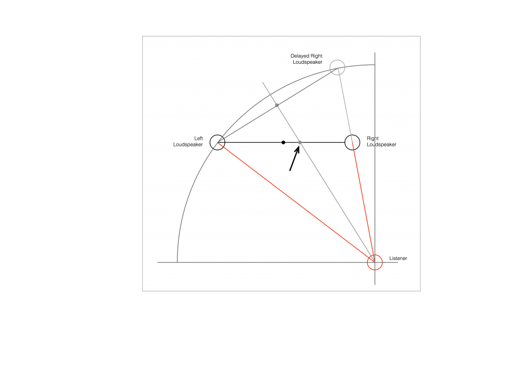
Notice that, after “correction”, the phantom image is still pulling towards the closer loudspeaker.
As we saw above, in order to push a phantom centre image towards a loudspeaker, you have to make the sound in that loudspeaker earlier.
So, what we need to do, after the distance-based time alignment is done, is to force the more distant loudspeaker to be a little earlier than the closer one. That will pull the phantom image towards it.
In order to use a distance compensation to make a loudspeaker produce the sound earlier, we have to tell the processor that it’s further away than it actually is. This makes the processor “think” that it needs to send the sound out early to compensate for the extra propagation delay caused by the distance.
So, to make the further loudspeaker a little early relative to the other loudspeaker, we either have to tell the processor that it’s further away from the listening position than it really is, or we reduce the reported distance to the closer loudspeaker to delay it a little more.
This means that, in the example shown in Figure 7, above, we should add a little to the distance to the left loudspeaker before entering the value in the menus, or subtract a little from the distance to the right loudspeaker instead.
How much is enough?
You might, at this point, be asking yourself “Why can’t this be done automatically? It’s just a little trigonometry, after all…”
If things were as simple as I’ve described here, then you’d be right – the math that is converting distance compensation to audio delays could include this offset, and everything would be fine.
The problem is that I’ve over-simplified a little on the way through. For example, not everyone hears exactly a 10º shift in phantom image with a 2.5 dB inter-channel amplitude difference. Those numbers are the average of a listening test with a number of subjects. Also, when other researchers have done the same test, they get slightly different results. (see this page for information).
Also, the directivity of the loudspeaker will have an influence (that is likely going to be frequency-dependent). So, if you’ve “toed in” your loudspeakers, then (in the example above) the further one will be “aimed” at you better than the closer one, which will have an influence on the perceived location of the phantom centre.
So, the only way to really do the final “tweaking” or “fine tuning” of the distance-compensation delays is to do it by listening.
Normally, I start by entering the distances correctly. Then, while sitting in the listening position, I use a monophonic track (Suzanne Vega singing “Tom’s Diner” works well) and I increase the distance in the surround processor’s menu of the loudspeaker that I want to pull the image towards. In other words, if the phantom centre appears to be located too far to the left, I “lie” to the surround processor and tell it that the right loudspeaker is further by 10 cm. I keep adding distance until the image is moved to the correct location.
Doppler demo
It’s obviously fake – but it’s a demo nonetheless…