B&O Tech: Near… Far…

#27 in a series of articles about the technology behind Bang & Olufsen loudspeakers

Introduction

To begin with, please watch the following video.

One thing to notice is how they made Grover sound near and far. Two things change in his voice (yes, yes, I know. It’s not ACTUALLY Grover’s voice. It’s really Yoda’s). The first change is the level – but if you’re focus on only that you’ll notice that it doesn’t really change so much. Grover is a little louder when he’s near than when he’s far. However, there’s another change that’s more important – the level of the reverberation relative to the level of the “dry” voice (what recording engineers sometimes call the “wet/dry mix”). When Grover is near, the sound is quite “dry” – there’s very little reverberation. When Grover is far, you hear much more of the room (more likely actually a spring or a plate reverb unit, given that this was made in the 1970’s).

This is a trick that has been used by recording engineers for decades. You can simulate distance in a mix by adding reverb to the sound. For example, listen to the drums and horns in the studio version of Penguins by Lyle Lovett. Then listen to the live version of the same people playing the same tune. Of course, there are lots of things (other than reverb) that are different between these two recordings – but it’s a good start for a comparison. As another example, compare this recording to this recording. Of course, these are different recordings of different people singing different songs – but the thing to listen for is the wet/dry mix and the perception of distance in the mix. Another example is this recording compared to this recording.

So, why does this trick work? The answer lies inside your brain – so we’ll have to look there first.

Distance Perception in the Mix

If you’re in a room with your eyes closed, and someone in the room starts talking to you, you’ll be pretty good at estimating where they are in the room – both in terms of angular location (you can point at them) and distance. This is true, even if you’ve never been in the room before. Very generally speaking, what’s going on here is that your brain is automatically comparing:

  • the two sounds coming into your two ears – the difference between these two signals tells you a lot about which direction the sound is coming from, AND
  • the direct sound from the source to the reflected sound coming from the room. This comparison gives you lots of information about a sound source’s distance and the size and acoustical characteristics of the room itself.

If we do the same thing in an anechoic chamber (a room where there are no echoes, because the walls absorb all sound) you will still be good at estimating the angle to the sound source (because you still have two ears), but you will fail miserably at the distance estimation (because there are no reflections to help you figure this out).

If you want to try this in real life, go outside (away from any big walls), close your eyes, and try to focus on how far away the sound sources appear to be. You have to work a little to force yourself to ignore the fact that you know where they really are  – but when you do, you’ll find that things sound much closer than they are. This is because outdoors is relatively anechoic. If you go to the middle of a frozen lake that’s covered in fluffy snow, you’ll come as close as you’ll probably get to an anechoic environment in real life. (unless you do this as a hobby)

So, the moral of the story here is that, if you’re doing a recording and you want to make things sound far away, add reflections and reverberation – or at least make them louder and the direct sound quieter.

Distance Perception in the Listening Room

Let’s go back to that example of the studio recording of Lyle Lovett recording of Penguins. If you sit in your listening room and play that recording out of a pair of loudspeakers, how far away do the drums and horns sound relative to you? Now we’re not talking about whether one sounds further away than the other within the mix. I’m asking, “If you close your eyes and try to guess how far away the snare drum is from your listening position – what would you guess?”

For many people, the answer will be approximately as far away as the loudspeakers. So, if your loudspeakers are 3 m from the listening position, the horns (in that recording) will sound about 3 m away as well. However, this is not necessarily the case. Remember that the perception of distance is dependent on the relative levels of the direct and reflected sounds at your ears. So, if you listen to that recording in an anechoic chamber, the horns will sound closer than the loudspeakers (because there are no reflections to tell you how far away things are). The more reflective the room’s surfaces, the more the horns will sound further away (but probably no further than the loudspeakers, since the recording is quite dry).

This effect can also be the result of the width of the loudspeaker’s directivity. For example, a loudspeaker that emits a very narrow beam (like a laser, assuming that were possible) would not send any sound towards the walls – only towards the listening position. So, this would have the same effect as having no reflection (because there is no sound going towards the sidewalls to reflect). In other words, the wider the dispersion of the sound from the loudspeaker (in a reflective room) the greater the apparent distance to the sound (but no greater than the distance to the loudspeakers, assuming that the recording is “dry”).

Loudspeaker directivity

So, we’ve established that the apparent distance to a phantom image in a recording is, in part, and in some (perhaps most) cases, dependent on the loudspeaker’s directivity. So, let’s concentrate on that for a bit.

Let’s build a very simple loudspeaker. It’s a model that has been used to simulate the behaviour of a real loudspeaker, so I don’t feel too bad about over-simplifying too much here. We’ll build an infinite wall with a piston in it that moves in and out. For example:

Here, you can see the piston (in red) moving in and out of the wall (in grey) with the resulting sound waves (the expanding curves) moving outwards in the air (in white).

The problem with this video is that it’s a little too simple. We also have to consider how the sound radiation off the front of the piston will be different at different frequencies. Without getting into the physics of “why” (if you’re interested in that, you can look here or here or here for an explanation) a piston has a general behaviour with repeat to the radiation patten of the sound wave it generates. Generally, the higher the frequency, the narrower the “beam” of sound. At low frequencies, there is basically no beam – the sound is emitted in all directions equally. At high frequencies, the beam to be very narrow.

The question then is “how high a frequency is ‘high’?” The answer to that lies in the diameter of the piston (or the diameter of the loudspeaker driver, if we’re interested in real life). For example, take a look at Figure 1, below.

Radiation of 100 Hz (blue) and 1.5 kHz (green) from a 10" diameter piston (i.e. a woofer).
Fig 1: Radiation of 100 Hz (blue) and 1.5 kHz (green) from a 10″ diameter piston (i.e. a woofer).

Figure 1 shows how loud a signal will be if you measure it at different directions relative to the face of a piston that is 10″ (25.4 cm) in diameter. Two frequencies are shown – 100 Hz (the blue curve) and 1.5 kHz (the green curve). Both curves have been normalised to be the same level (100 dB SPL – although the actual value really doesn’t matter) on axis (at 0°). As you can see in the plot, as you move off to the side (either to 90° or 270°) the blue curve stays at 100 dB SPL. So, no matter what your angle relative to on-axis to the woofer, 100 Hz will be the same level (assuming that you maintain your distance). However, look at the green curve in comparison. As you move off to the side, the 1.5 kHz tone drops by more than 20 dB. Remember that this also means that (if the loudspeaker is pointing at you and the sidewall is to the side of the loudspeaker) then 100 Hz and 1.5 kHz will both get to you at the same level. However, the reflection off the wall will have 20 dB more level at 100 Hz than at 1.5 kHz. This also means, generally, that there is more energy in the room at 100 Hz than there is at 1.5 kHz because, if you consider the entire radiation of the loudspeaker averaged over all directions at the same time the lower frequency is louder in more places.

This, in turn, means that, if all you have is a 10″ woofer and you play music, you’ll notice that the high frequency content sounds closer to you in the room than the low frequency content.

If the loudspeaker driver is smaller, the effect is the same, the only difference is that the effect happens at a higher frequency. For example, Figure 2, below shows the off-axis response for two frequencies emitted by a 1″ (2.54 cm) diameter piston (i.e. a tweeter).

Radiation of 1.5 kHz (blue) and 15 kHz (green) from a 1" diameter piston (i.e. a tweeter).
Radiation of 1.5 kHz (blue) and 15 kHz (green) from a 1″ diameter piston (i.e. a tweeter).

Notice that the effect is identical, however, now, 1.5 kHz is the “low frequency region for the small piston, so it radiates in all directions equally (seen as the blue curve). The high frequency (now 15 kHz) becomes lower and lower in level as you move off to the side of the driver, going as low as -20 dB at 90°.

So, again, if you’re listening to music through that tweeter, you’ll notice that the frequency content at 1.5 kHz sounds further away from the listening position than the content at 15 kHz. Again, the higher the frequency, the closer the image.

Same information, shown differently

If you trust me, figures 1 and 2, above, show you that the sound radiating off the front of a loudspeaker driver gets narrower with increasing frequency. If you don’t trust me (and you shouldn’t – I’m very untrustworthy…) then you’ll be saying “but you only showed me the behaviour at two frequencies… what about the others?” Well, let’s plot the same basic info differently, so that we can see more data.

Figure 3, below, shows the same 10″ woofer, although now showing all frequencies from 20 Hz to 20 kHz, and all angles from -90° to +90°. However, now, instead of showing all levels (in dB) we’re only showing 3 values, at -1 dB, -3 dB, and -10 dB. ( These plots are a little tougher to read until you get used to them. However, if you’re used to looking at topographical maps, these are the same.)

A contour plot showing the directivity of a 10" piston (i.e. a woofer). The red area has a magnitude between 0 and -1 dB. The orange area has a magnitude of -1 down to -3 dB. The blue area has a magnitude of -3 down to -10 dB. The white area is lower than -10 dB.
Fig 3: A contour plot showing the directivity of a 10″ piston (i.e. a woofer). The red area has a magnitude between 0 and -1 dB. The orange area has a magnitude of -1 down to -3 dB. The blue area has a magnitude of -3 down to -10 dB. The white area is lower than -10 dB.

Now you can see that, as you get higher in frequency, the angles where you are within 1 dB of the on-axis response gets narrower, starting at about 400 Hz. This means that a 10″ diameter piston (which we are pretending to be a woofer) is “omnidirectional” up to 400 Hz, and then gets increasingly more directional as you go up.

Figure 4 shows the same information for a 1″ diameter piston. Now you can see that the driver is omnidirectional up to about 4 kHz. (This is not a coincidence – the frequency is 10 times that of the woofer because the diameter is one tenth.)

A contour plot showing the directivity of a 1" piston (i.e. a tweeter). The red area has a magnitude between 0 and -1 dB. The orange area has a magnitude of -1 down to -3 dB. The blue area has a magnitude of -3 down to -10 dB. The white area is lower than -10 dB.
Fig 4: A contour plot showing the directivity of a 1″ piston (i.e. a tweeter). The red area has a magnitude between 0 and -1 dB. The orange area has a magnitude of -1 down to -3 dB. The blue area has a magnitude of -3 down to -10 dB. The white area is lower than -10 dB.

Normally, however, you do not make a loudspeaker out of either a woofer or a tweeter – you put them together to cover the entire frequency range. So, let’s look at a plot of that behaviour. I’ve put together our two pistons using a 4th-order Linkwitz-Riley crossover at 1.5 kHz. I have also not included any weirdness caused by the separation of the drivers in space. This is theoretical world where the tweeter and the woofer are in the same place  – an impossible coaxial loudspeaker.

A contour plot showing the directivity of a two-way loudspeaker made of a 1" and a 10" piston. The red area has a magnitude between 0 and -1 dB. The orange area has a magnitude of -1 down to -3 dB. The blue area has a magnitude of -3 down to -10 dB. The white area is lower than -10 dB.
Fig 5: A contour plot showing the directivity of a two-way loudspeaker made of a 1″ and a 10″ piston. The red area has a magnitude between 0 and -1 dB. The orange area has a magnitude of -1 down to -3 dB. The blue area has a magnitude of -3 down to -10 dB. The white area is lower than -10 dB.

In Figure 5 you can see the effects of the woofer’s directivity starting to beam below the crossover, and then the tweeter takes over and spreads the radiation wide again before it also narrows.

So what?

Why should you care about understanding the plot in Figure 5? Well, remember that the narrower the radiation of a loudspeaker, the closer the sound will appear to be to you. This means that, for the imaginary loudspeaker shown in Figure 5, if you’re playing a recording without additional reverberation, the low frequency stuff will sound far away (the same distance as the loudspeakers), So will a narrow band between 3 kHz and 4 kHz (where the tweeter pulls the radiation wider). However, the materials in the band around 700 Hz – 2 kHz and in the band above 7 kHz will sound much closer to you.

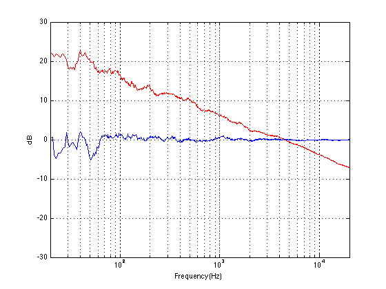
Another way to express this is to show a graph of the resulting level of the reverberant energy in the listening room relative to the direct sound, an example of which is shown in Figure 6. (This is a plot copied from “Acoustics and Psychoacoustics” by David Howard and Jamie Angus).

Reverberant energy from the room relative to the direct sound from a two-way loudspeaker. (X and Angus, 2000)
Fig 6: Reverberant energy from the room relative to the direct sound from a two-way loudspeaker. (from Howard and Angus, 2000)

This shows a slightly different loudspeaker with a crossover just under 3 kHz. This is easy to see in the plot, since it’s where the tweeter starts putting more sound into the room, thus increasing the amount of reverberant energy.

What does all of this mean? Well, if we simplify a little, it means that things like voices will pull apart in terms of apparent distance. Consonant sounds like “s” and “t” will appear to be closer than vowels like “ooh”.

So, whaddya gonna do about it?

All of this is why one of the really important concerns of the acoustical engineers at Bang & Olufsen is the directivity of the loudspeakers. In a previous posting, I mentioned this a little – but then it was with regards to identifying issues related to diffraction. In that case, directivity is more of a method of identifying a basic problem. In this posting, however, I’m talking about a fundamental goal in the acoustical design of the loudspeaker.

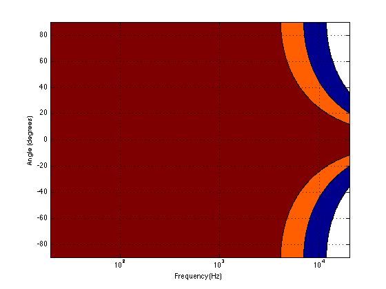
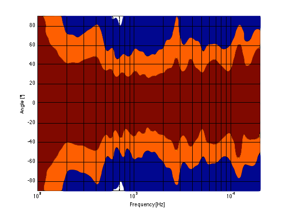
For example, take a look at Figures 7 and 8 and compare them to Figure 9. It’s important to note here that these three plots show the directivities of three different loudspeakers with respect to their on-axis response. The way this is done is to measure the on-axis magnitude response, and call that the reference. Then you measure the magnitude response at a different angle, and then calculate the difference between that and the reference. In essence, you’re pretending that the on-axis response is flat. This is not to be interpreted that the three loudspeakers shown here have the same on-axis response. They don’t. Each is normalised to its own on-axis response. So we’re only considering how the loudspeaker compares to itself.

A contour plot showing the directivity of a commercially available 3-way loudspeaker. The red area has a magnitude between 0 and -1 dB. The orange area has a magnitude of -1 down to -3 dB. The blue area has a magnitude of -3 down to -10 dB. The white area is lower than -10 dB.
Fig 7: A contour plot showing the directivity of a commercially available 3-way loudspeaker. The red area has a magnitude between 0 and -1 dB. The orange area has a magnitude of -1 down to -3 dB. The blue area has a magnitude of -3 down to -10 dB. The white area is lower than -10 dB.

Figure 7, above, shows the directivity behaviour of a commercially-available 3-way loudspeaker (not from Bang & Olufsen). You can see that the woofer is increasingly beaming (the directivity gets narrow)  up to the 3 – 5 kHz area. The midrange is beaming up above 10 kHz or so. So, a full band signal will sound distant in the low end, in the 6-7 kHz range and around 15 kHz. By comparison, signals at 2-4 kHz and 10-15 kHz will sound quite close.

A contour plot showing the directivity of traditionally designed 4-way loudspeaker. The red area has a magnitude between 0 and -1 dB. The orange area has a magnitude of -1 down to -3 dB. The blue area has a magnitude of -3 down to -10 dB. The white area is lower than -10 dB.
Fig 8: A contour plot showing the directivity of traditionally designed 4-way loudspeaker. The red area has a magnitude between 0 and -1 dB. The orange area has a magnitude of -1 down to -3 dB. The blue area has a magnitude of -3 down to -10 dB. The white area is lower than -10 dB.

Figure 8, above, shows the directivity behaviour of a 3-way loudspeaker we made as a rough prototype. This is just a woofer, midrange and tweeter, each in its own MDF box – nothing fancy – except that the tweeter box is not as wide as the midrange box which is narrower than the woofer box. You can see that the woofer is beaming (the directivity gets narrow)  just above 1 kHz – although it has a very weird wide directivity at around 650 Hz for some reason. The midrange is beaming up from 5kHz to 10 kHz, and then the tweeter gets wide. So, this loudspeaker will have the same problem as the commercial loudspeaker

A contour plot showing the directivity of a BeoLab 5. The red area has a magnitude between 0 and -1 dB. The orange area has a magnitude of -1 down to -3 dB. The blue area has a magnitude of -3 down to -10 dB. The white area is lower than -10 dB.
Fig 9: A contour plot showing the directivity of a BeoLab 5. The red area has a magnitude between 0 and -1 dB. The orange area has a magnitude of -1 down to -3 dB. The blue area has a magnitude of -3 down to -10 dB. The white area is lower than -10 dB.

As you can see, the loudspeaker with the directivity shown in Figure 9 (the BeoLab 5) is much more constant as you change frequency (in other words, the lines are more parallel). It’s not perfect, but it’s a lot better than the other two – assuming that constant directivity is your goal. You can also see that the level of the signal that is within 1 dB of the on-axis response is quite wide compared with the loudspeakers in Figures 7 and 8. The loudspeaker in Figure 7 not only beams in the high frequencies, but also has some strange “lobes” where things are louder off-axis than they are on-axis (the red lines).

When you read B&O’s marketing materials about the reason why we use Acoustic Lenses in our loudspeakers, the main message is that it’s designed to spread the sound – especially the high frequencies – wider than a normal tweeter, so that everyone on the sofa can hear the high hat. This is true. However, if you ask one of the acoustical engineers who worked on the project, they’ll tell you that the real reason is to maintain constant directivity as well as possible in order to ensure that the direct-to-reverberant ratio in your listening room does not vary with frequency. However, that’s a difficult concept to explain in 1 or 2 sentences, so you won’t hear it mentioned often. However, if you read this paper (which was published just after the release of the BeoLab 5), for example, you’ll see that it was part of the original thinking behind the engineers on the project.

 Addendum 1.

I’ve been thinking more about this since I wrote it. One thing that I realised that I should add was to draw a comparison to timbre. When you listen to music on your loudspeakers in your living room, in a best-case scenario, you hear the same timbral balance that the recording engineer and the mastering engineer heard when they worked on the recording. In theory, you should not hear more bass or less midrange or more treble than they heard. The directivity of the loudspeaker has a similar influence – but on the spatial performance of the loudspeakers instead of the timbral performance. You want a loudspeaker that doesn’t alter the relative apparent distances to sources in the mix – just like you don’t want the loudspeakers to alter the timbre by delivering too much high frequency content.

Addendum 2.

One more thing… I made the plot below to help simplify the connection between directivity and Grover. Hope this helps.

A contour plot showing the directivity of a commercially available 3-way loudspeaker. The wider the plot (vertically), the farther the image.

Audio Mythinformation: 16 vs 24 bit recordings

Preface: Lincoln was right

There is a thing called “argument from authority” which is what happens when you trust someone to be right about something because (s)he knows a lot about the general topic. This is used frequently by pop-documentaries on TV when “experts” are interviewed about something. Example: “we asked an expert in underwater archeology how this piece of metal could wind up on the bottom of the ocean, covered in mud and he said ‘I don’t know’ so it must have been put there by aliens millions of years ago.” Okay, I’m exaggerating a little here, but my point is that, just because someone knows something about something, doesn’t mean that (s)he knows everything about it, and will always give the correct answers for every question on the topic.

In other words, as Abraham Lincoln once said: “Don’t believe everything you read on the Internet.”

Of course, that also means that also applies to everything that follows in the posting below (arrogantly assuming that I can be considered to be an authority on anything), so you might as well stop reading and go do something useful.

My Inspiration

There has been some discussion circulating around the Interweb lately about the question of whether the “new” trend to buy “high-resolution” audio files with word lengths of 24 bits actually provides an improvement in quality over an audio file with “only” 16 bits.

One side of this “religious” war comes from the people who are selling the high-res audio files and players. The assumed claim is that 24 bits makes a noticeable improvement in audio quality (over a “mere” 16 bits) that justifies asking you to buy the track again – and probably at a higher price.

The other side of the war are bloggers and youtube enthusiasts who write things like (a now-removed) article called “24/192 Music Downloads… and why they make no sense” (which, if you looked at the URL, is really an anti-Pono rant) and “Bit Depth & The 24 Bit Audio Myth

Personally, I’m not a fan of religious wars, so I’d like to have a go at wading into the waters in a probably-vain attempt to clear up some of the confusion and animosity that may be caused by following religious leaders.

Some background

If you don’t know anything about how an audio signal is converted from analogue to digital, you should probably stop reading here and go check out this page or another page that explains the same thing in a different way.

Now to recap what you already know:

  • An analogue to digital converter makes a measurement of the instantaneous voltage of the audio signal and outputs that measurement as a binary number on each “sample”
  • The resolution of that converter is dependent on the length of the binary number it outputs. The longer the number, the higher the resolution.
  • The length of a binary number is expressed in Binary digITs or BITS.
  • The higher the resolution, the lower the noise floor of the digital signal.
  • In order to convert the artefacts caused by quantisation error from distortion to program-dependent noise, dither is used. (Note that this is incorrectly called “quantisation noise” by some people)
  • In a system that uses TPDF (Triangular Probability Distribution Function) dither, the noise has a white spectrum, meaning that is has equal energy per Hz.

A good rule of thumb in a PCM system with TPDF dithering is that the dynamic range of the system is approximately 6 * the number of bits – 3 dB. For example, the dynamic range of a 16-bit system is 6*16-3 = 93 dB. Some people will say that this is the signal-to-noise ratio of the system, however, this is only correct if your signal is always as loud as it can be.

Let’s think about what, exactly, we’re saying here. When we measure the dynamic range of a system, we’re trying to find out what the difference is (in dB) between (1) the loudest sound you can put through the system without clipping and (2) the noise floor of the system.

The goal of an engineer when making a piece of audio gear (or of a recording engineer when making a recording) is to make the signal (the music) so loud that you can’t hear the noise – but not so loud that the signal clips and therefore distorts. There are three ways to improve this: you can either (1) make your gear capable of making the signal louder, (2) design your gear so that it has less noise, or (3) both of those things. In either case, what you are trying to maximise is the ratio of the signal to the noise. In other words, relative to the noise level, you want the signal as high as possible.

However, this is a rather simplistic view of the world that has two fatal flaws:

The first problem is that (unless you like most of the music my kids like) the signal itself has a dynamic range – it gets loud and it also gets quiet. This can happen over long stretches of time (say, if you’re listening to a choral piece written by Arvo Pärt) or over relatively short periods of time (say, the difference between the sharp peak of a rim shot on a snare and the decay of a piano noise in the middle of the piece of music I’ve plotted below.)

You should note that this isn’t a piece that I use to demonstrate wide dynamic range or anything – I just started looking through my classical music collection for a piece that can demonstrate that music has loud AND quiet sections – and this was the second piece I opened (it’s by the Ahn Trio – I was going alphabetically…) So don’t make a comment about how I searched for an exceptional example of the once recording in the history of all recordings that has dynamic range. That would be silly. If I wanted to do that, I would have dug out an Arvo Pärt piece – but Arvo comes after Ahn in the alphabet, so I didn’t get that far.

Screenshot of a a piece of music by the Ahn Trio.
Figure 1: Screenshot of the waveform representation of the Concerto for Piano Trio and Percussion, performed by the Ahn Trio. Note how big the difference is between the peaks and the quiet sections.

The portion of this piece that I’ve highlighted in Figure 1 (the gray section in the middle) has a peak at about 1 dB below full scale, and, at the end gets down to about -46 dB below that. (You might note that there is a higher peak earlier in the piece – but we don’t need to worry about that.) So, that little portion of the music has a dynamic range of about 45 dB or so – if we’re just dumbly looking at the plot.

So, this means that we want to have a recording system and a playback system for this piece of music that has can handle a signal as loud as that peak without distorting it – but has a constant noise floor that is quiet enough that I won’t hear it at the end of that piano note decaying at the end of that little section I’ve highlighted.

What we’re really talking about here is more accurately called the dynamic range of the system (and the recording). We’re only temporarily interested in the Signal to Noise ratio, since the actual signal (the music) has a constantly varying level. What’s more useful is to talk about the dynamic range – the difference  (in dB) between the constant noise of the system (or the recording) and the maximum peak it can produce. However, we’ll come back to that later.

The second problem is that the noise floor caused by TPDF dither is white noise, which means that you have equal energy per Hertz as we’ve seen before. We can also reasonably safely assume that the signal is music which usually consists of a subset of all frequencies at any moment in time (if it had all frequencies present, it would sound like noise of some colour instead of Beethoven or Bieber), that are probably weighted like pink noise – with less and less energy in the high frequencies.

In a worst-case situation, you have one note being played by one instrument and you’re hoping that that one note is going to mask (or “drown out”) the noise of the system that is spread across a very wide frequency range.

For example, let’s look again at the decay of that piano note in the example in Figure 1. That’s one note on a piano, dropping down to about -40-something dB FS, with a small collection of frequencies (the fundamental frequency of the pitch and its multiples), and you’re hoping that this “signal” is going to be able to mask white noise that stretches in frequency band from something below 20 Hz all the way up past 20 kHz. This is worrisome, at best.

In other words, it would be easy for a signal to mask a noise if the signal and the noise had the same bandwidth. However, if the signal has a very small bandwidth and the noise has a very wide bandwidth, then it is almost impossible for the signal to mask the noise.

In other words, the end of the decay of one note on a piano is not going to be able to cover up hiss at 5 kHz because there is no content at 5 kHz from the piano note to do the covering up.

So, what this means is that you want a system (either a recording or a piece of audio gear) where, if you set the volume such that the peak level is as loud as you want it to be, the noise floor of the recording and the playback system is inaudible at the listening position. (We’ll come back to this point at the end.) This is because the hope that the signal will mask the noise is just that – hope. Unless you listen to “music” that has no dynamic range and is constantly an extremely wide bandwidth, then I’m afraid that you may be disappointed.

One more thing…

There is another assumption that gets us into trouble here – and that is the one I implied earlier which says that all of my audio gear has a flat magnitude response. (I implied it by saying that we can assume that the noise that we get is white.)

Let’s look at the magnitude response of a pair of earbud headphones that millions and millions of people own. I borrowed this plot from this site – but I’m not telling you which earbuds they are – but I will say that they’re white. It’s the top plot in Figure 2.

Top plot: The frequency response of a pair of earbud headphones. Bottom plot: The magnitude response of a filter I made to "copy" the response.
Fig 2: Top plot: The magnitude response of a pair of earbud headphones. Bottom plot: The magnitude response of a filter I made to mimic the response. It’s not perfect – but it’s close enough for the arguments I’m making here.

This magnitude response is a “weighting” that is applied to everything that gets into the listener’s ears (assuming that you trust the measurement itself). As you can see if you put in a signal that consists of a 20 Hz tone and a 200 Hz tone that are equal in level, then you’ll hear the 200 Hz tone about 40 dB louder than the 20 Hz tone. Remember that this is what happens not only to the signal you’re listening to, but also the noise of the system and the recording – and it has an effect.

For example, if we measure a 16-bit linear PCM digital system with TPDF dithering, we’ll see that it has a 93.3 dB dynamic range. This means that the RMS level of a sine wave (or another signal) that is just below clipping the system (so it’s as loud as you can get before you start distorting) is 93.3 dB louder than the white noise noise floor (yes, the repetition is intentional – read it again). However, that is the dynamic range if the system has a magnitude response that is +/- 0 dB from 0 Hz to half the sampling rate.

If, however, you measured the dynamic range through those headphones I’m talking about in Figure 2, then things change. This is because the magnitude response of the headphones has an effect on both the signal and the noise. For example, if the signal you used to measure the maximum capabilities of the system were a 3 kHz sine tone, then the dynamic range of the system would improve to about 99 dB. (I measured this using the filter I made to “fake” the magnitude response – it’s shown in the bottom of Figure 2.)

Remember that, with a flat magnitude response, the dynamic range of the 16-bit system is about 93 dB. By filtering everything with a weird filter, however, that dynamic range changes to 99 dB IF THE SIGNAL WE USE TO MEASURE THE SYSTEM IS a 3 kHz SINE TONE.

The problem now is that the dynamic range of the system is dependent on the spectrum of the signal we use to measure the peak level with – which will also be true when we consider the signal to noise ratio of the same system. Since the spectrum of the music AND the dither noise are both filtered by something that isn’t flat, the SNR of the system is dependent on the frequency content of the music and how that relates to the magnitude response of the system.

For example, if we measured the dynamic range of the system shown above using sine tones at different frequencies as our measurement signal, we would get the values shown in Figure 3

The dynamic range of a 16-bit TPDF system, if the measurement is done relative to a sine wave.
Fig 3: The dynamic range of a 16-bit TPDF system that includes the filter shown in the bottom of Figure 2, if the measurement is done relative to a sine wave with a frequency shown in the x-axis.

If you’re looking not-very-carefully-at-all at the curve in Figure 3, you’ll probably notice that it’s basically the curve on the bottom of Figure 2, upside down. This makes sense, since, generally, the filter will attenuate the total power of the noise floor, and the signal used to make the dynamic range measurement is a sine wave whose level is dependent on the magnitude response. What this means is that, if your system is “weak” at one frequency band, then the signal to noise ratio of the system when the signal consists of energy in the “weak” band will be worse than in other bands.

Another way to state this is: if you own a pair of those white earbuds, and you listen to music that only has bass in it (say, the opening of this tune) you might have to turn up the level so much to hear the bass that you’ll hear the noise floor in the high end.

Wrapping up

As I said at the beginning, some people say “more bits are better, so you should buy all your music again with 24-bit versions of your 16-bit collection”. Some other people say “24-bits is a silly waste of money for everyone”.

What’s the truth? Probably neither of these. Let’s take a couple of examples to show that everyone’s wrong.

Case 1: You listen to music with dynamic range and you have a good pair of loudspeakers that can deliver a reasonably high peak SPL level. You turn up the volume so that the peak reaches, say, 110 dB SPL (this is loud for a peak, but if it only happens now and again, it’s not that scary). If your recording is a 16-bit recording, then the noise floor is 93 dB below that,  so you have a wide-band noise floor of 17 dB SPL which is easily audible in a quiet room. This is true even when the acoustic noise floor of the room is something like 30 dB SPL or so, since the dither noise from the  loudspeaker has a white noise characteristic, whereas acoustic background noise in “real life” is usually pink in spectrum. So, you might indeed hear the high-frequency hiss. (Note that this is even more true if you have a playback system with active loudspeakers that protect themselves from high peaks – they’ll reduce the levels of the peaks, potentially causing you to push up the volume knob even more, which brings the noise floor up with it.)

The FFT's of a white noise sample (the blue curve) and a pink noise sample (the red curve), both of which have the same total RMS level.
Fig 4: The FFT’s of a white noise sample (the blue curve) and a pink noise sample (the red curve), both of which have the same total RMS level.

Case 2: You have a system with a less-than-flat magnitude response (i.e. a bass roll-off) and you are listening to music that only has content in that frequency range (i.e. the bass), so you turn up the volume to hear it. You could easily hear the high-frequency noise content in the dither if that high frequency is emphasised by the playback system.

Case 3: You’re listening to your tunes that have no dynamic range (because you like that kind of music) over leaky headphones while you’re at the grocery store shopping for eggs. In this case, the noise floor of the system will very likely be completely inaudible due to the making by the “music” and the background noise of announcements of this week’s specials.

The Answer

So, hopefully I’ve shown that there is no answer to this question. At least, there is no one-size-fits-all answer. For some people, in some situations, 16 bits are not enough. There are other situations where 16 bits is plenty. The weird thing that I hope that I’ve demonstrated is that the people who MIGHT benefit from higher resolution are not necessarily those with the best gear. In fact, in some cases, it’s people with worse gear that benefit the most…

… but Abraham Lincoln was definitely right. Stick with that piece of advice and you’ll be fine.

Appendix 1: Noise shaping

One of the arguments against 24-bit recordings is that a noise-shaped 16-bit recording is just as good in the midrange. This is true, but there are times when noise shaping causes playback equipment some headaches, since it tends to push a lot of energy up into the high frequency band where we might be able to hear it (at least that’s the theory). The problem is that the audio gear is still trying to play that “signal”, so if you have a system that has issues, for example, with Intermodulation Distortion (IMD) with high-frequency content (like a cheap tweeter, as only one example) then that high-frequency noise may cause signals to “fold down” into audible bands within the playback gear. So noise shaping isn’t everything it’s cracked up to be in some cases.

We are not amused

If you don’t own a 2011-model Apple MacBook Pro with a problem with it’s discrete GPU, then you should probably stop reading right now and go look at a video on wimp.com instead. This one is pretty funny.


The backstory

I confess. I’m a Macintosh person. In fact, I’m one of those annoying Mac people who makes fun of people who own Windows machines. I’ve been a Mac person since about 1990 when I bought my first computer – a Mac Classic. In those days, if you used a computer for MIDI, you had to get a Mac because Windows machines never really knew what time it was. Not precisely or accurately enough to be used to play a MIDI file. And, once audio editing came along (not ProTools – the GOOD stuff, like Sonic Solutions) it was Macintosh or nothing because Windows people would look at you funnily when you talked about SCSI drives.

Last week, though, my evangelism came to a crashing halt when my trusty 2-year old MacBook Pro suddenly went bezerk. It started with my son booting up Minecraft, which tried to change the screen resolution. The result was a large black vertical stripe down the middle of the screen with the left side of the desktop on the right side of the screen, wrapping around to the left side. “Dad, there’s something wrong with the computer…” he said. “No problem” I said, “let’s just reboot it.”

Rebooted the computer, got the pretty grey Apple logo, then just a blank grey screen. Tried again, same result, Tried again, same result… Uh oh… It’s only been a couple of weeks since the last backup, so I haven’t lost too much data – but the time it’s going to take to get up and running again… Guh.

So, I started Googling for some solutions about what to do with a stuck grey screen. Apple has a friendly page about this – try this, try that… If that doesn’t work, try something else. If that doesn’t work, you probably have to reformat your drive. Guh.

Then I Googled some more and found out that my symptoms were not unusual. In fact, it wasn’t long before I came across a news article and another one and a very long discussion thread on the Apple Users Forum with over 1,000,000 views and an online petition (currently standing at over 13,000 signatures) – where everybody was talking about me – or at least my problem with my Mac.

Turns out that my hard drive is fine. My data is all intact. What is NOT fine is my discrete Graphic Processor Unit or GPU. Apparently, MacBook Pro’s made in 2011 (mine is a late-2011 model) are dropping like flies. And, interestingly, the whole mess was sort of predicted by this site when they did a tear-down of the computer back when it first came out. As they said back then, in talking about the GPU: “Holy thermal paste! Time will tell if the gobs of thermal paste applied to the CPU and GPU will cause overheating issues down the road.” and “Absurd amounts of pre-applied thermal paste may cause problems down the road.”

Okay, so the MBP’s from 2011 have a problem. This is forgivable – even engineers make mistakes sometimes. Manufacturing or design defects are not surprising in this day and age. However, what astounds me is that Apple is completely denying that this issue exists.The stories being told tell tales of people forking out over $300 to get a logic board replacement, only to have it fail within a couple of months. Another $300 logic board, also fails… Apparently, Apple is replacing faulty logic boards with “refurbished” boards that have exactly the same problem as the one getting taken out of the machine. So it seems that there is a large circulation of faulty circuit boards getting put into machines at $300 a pop. This means that I won’t be sending my computer off to get a “new” logic board any time soon.

Solution #1

Other people tell epic tales of a great little utility called gfxCardStatus which allows you to force the computer into using either the discrete GPU or the integrated GPU.

So, following some interactions on the Interweb, I tried rebooting my computer over and over and over and over (say, about 50 times, but it felt like a million…) until it worked! installed gfxCardStatus and locked it into the integrated GPU. Life was great. A little slow, but great. At least my computer was up and running again. Long enough to do a backup of EVERYTHING – just in case.

Sadly, the party didn’t last long. 4 days later, the machine crashed. 50 reboots later, it was running again – this time for only 3 days. And when it crashed that time, things got worse.  The machine did a complete shutdown, and restarting resulted in another complete shutdown immediately after seeing a stripy grey Apple sign.

Solution #2

So, I went to plan #2 – trying to disable the discrete GPU permanently by moving the .kext, .plugin and .bundle files for the GPU. I did this following the instructions at this page – which I’ve repeated below.  If you’re reading this because you have the same problem as I do, and you try this, don’t hold me responsible if you break your Mac using this technique. It was a last-ditch attempt for me to revive my machine – and so far so good…

  1. Start up in Single User Mode (hold down CMD-S immediately after startup)
  2. Get ready to move System files by typing the text mount -uw /
  3. Create a directory to move the Extension files into by typing mkdir /System/Library/DisabledExtensions
  4. Move the files by typing mv /System/Library/Extensions/ATI* /System/Library/DisabledExtensions
  5. Type exit
  6. You might need to type exit again to reboot.


This still required that I do a hard shutdown (holding the power button for 5 seconds) and restart 4 or 5 times – but here I am, once again, typing on my computer that, yesterday, was a brick. Let’s hope that this solution sticks.

However, what would be REALLY nice is if Apple were to own up to this one, and call up all those people like me who own a defective machine, and tell us that they’re going to fix it for free. Or at least fix it for a reasonable cost with a solution that actually works. Either way, I might regain a little faith in a company that I used to trust.


A little more information, in case you’re reading this because you have a similar problem: I have a 15″ late-2011 MacBook Pro with an AMD Radeon HD 6750M discrete GPU. I haven’t done anything to it (like replace the HD or add extra RAM).

For more information about this, see http://action.mbp2011.com.


Bang & Olufsen BeoVision Avant Reviews

bvavant


I was responsible for the final sound design (aka tonal balance) of the loudspeakers built into the BeoVision Avant. So, I’m happy to share some of the blame for some of the comments (at least on the sound quality) from the reviews.


from Home Cinema Choice magazine

“Where the Avant really gets space-age, though, is with … its ability to drive 21 audio channels ”

“This effort by the integrated speakers , together with its unprecedented audio flexibility,makes the Avant the finest sounding TV I’ve ever heard.”


from TrustedReviews.com

“Even a high-end sound bar would struggle to match the gorgeous finesse the Avant combines with its raw power. The speakers reproduce soundtrack subtleties more precisely and elegantly than any other TV we’ve heard. And they do so no matter how dense the soundstage becomes, and without so much as a hint of treble harshness.”

“Then there’s that rear-mounted subwoofer. We had worried that the way this angled subwoofer fires up and out through an actually quite narrow vent could cause boominess or distortion, but not a bit of it. Instead very impressive and well-rounded amounts of bass meld immaculately into the bottom end of the wide mid-range delivered by those terrific left, right and centre speakers.”


from flatpanelshd.com

Compared to all other TVs on the market (non-B&O) there is no competition. Sound is so much better. However, we also have to point out that the TV did not receive the best conditions for a proper audio demonstration.

Bang & Olufsen BeoLab 18 Reviews

xl_B&O-BeoLab-17-Close-624


I was part of the development team, and one of the two persons who decided on the final sound design (aka tonal balance) of the B&O BeoLab 18 loudspeakers. So, I’m happy to share some of the blame for some of the comments (at least on the sound quality) from the reviews.


Bernard Dickinson at Live Magazines said:

The sound reproduction is flawless”


Lyd & Billede’s August 2014 review said

“Lydkvaliteten er rigtig god med en åben, distinkt og fyldig gengivelse, som ikke gør højopløste lydformater til skamme.” (The sound quality is very good with an open, clear and detailed reproduction, which do not put high-resolution audio formats to shame.)

and ”Stemmerne er lige klare og tydelige, hvad enten vi sidder lige i smørhullet eller befinder os langt ude i siden. Det er faktisk ret usædvanligt og gør, at BeoLab 18 egner sig lige godt til både baggrundsmusik og aktiv lytning” (The voices are crisp and clear, whether we are sitting right in the sweet spot or far off to the side. It’s actually quite unusual and makes the BeoLab 18 equally suited for both background music and active listening)