This video shows the inner workings of an early electronic calculator. The cool thing is that it uses a delay-line memory based on an acoustic signal running down a length of steel.
Author: geoff
DFT’s Part 3: The Math
Links to:
DFT’s Part 1: Some introductory basics
DFT’s Part 2: It’s a little complex…
If you have an audio signal or the impulse response measurement of an audio device (which is just the audio output of a device when the input signal is a very short “click” – how the device responds to an impulse), one way to find out its spectral content is to use a Fourier Transform. Normally, we live in a digital audio world, with discrete divisions of time, so we use a DFT or a Discrete Fourier Transform (although most people call it an FFT – a Fast Fourier Transform).
If you do a DFT of a signal (say, a sinusoidal waveform), then you take a slice of time, usually with a length (measured in samples) that is a nice power of 2 – for example 2, or 4 (2^2), or 2^12 (4096 samples) or 2^13 (8192 samples). When you convert this signal in time through the DFT math, you get out the same number of number (so, 2048 samples in, 2048 numbers out). Each of those numbers can be used to find out the magnitude (the level) and the phase for a frequency.
Those frequencies (say, 2048 of them) are linearly spaced from 0 Hz up to just below the sampling rate (the sampling rate would be the 2049th frequency in this case… we’ll see why, below…)
So, generally speaking: if I have an audio signal (a measurement of level over time) and I do a DFT (which is just a series of mathematical equations) and then I can see the relative amount of energy by frequency for that “slice” of time.
So, how does the math work? In essence, it’s just a matter of doing a lot of multiplication, and then adding the results that you get (and then maybe doing a little division, if you’re in the mood…). We’ve already seen in Parts 1 and 2 of this series that
- a sinusoidal waveform is just 2 dimensions (dimension #1 is movement in space, the other dimension is time) of a three-dimensional rotation (dimensions #1 and #2 are space and #3 is time)
- if we want to know the frequency, the amplitude, and the direction of rotation of the “wheel”, we will need to see the real component (the cosine) and the imaginary component (the negative sine)
- the imaginary component is a negative sine wave instead of a positive sine wave because the wheel is rotation clockwise
A real-world example
I took a bell and I hit it, so it rang the way bells ring. While I was doing that, I recorded it with a microphone connected to my computer. The sampling rate was 48 kHz and I recorded with enough bits to not worry about that. The result of that recording is shown in Figure 1.

Seven seconds is a lot of samples at 48,000 samples per second. (In fact, it’s 7 * 48000 samples – which is a lot…) So, let’s take a slice somewhere out of the middle of that recording. This portion (a “zoomed-in” view of Figure 1) is shown below in Figure 2.

So, for the remainder of this posting, we’ll only be looking at that little slice of time, 2048 samples long. Since our sampling rate is 48 kHz, this means that the total length of that slice is 2048 * 1/48000 = 0.0427 seconds, or approximately 42.7 ms.
Let’s start by calculating the amount of energy there is at 0 Hz or “DC” in this section. We do this by taking the value of each individual sample in the section, and adding all those values together. Some of the values are positive (they’re above the 0 line in Figure 2) and some are negative (they’re below 0). So, if we add them all up we should be somewhere close to 0… Let’s try….
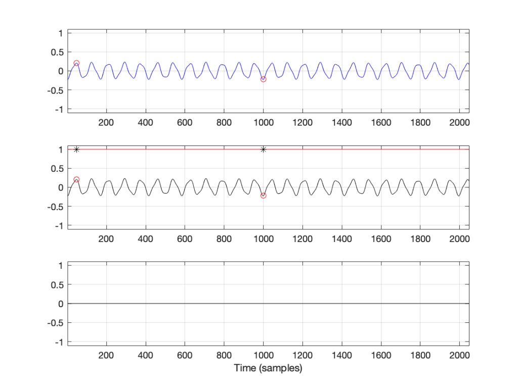
Figure 3 has three separate plots. The top plot in blue is the section of the recording that we’re using, 2048 samples long. You’ll see that I put a red circle around two samples, sample number 47 and sample number 1000. These were chosen at random, just so we have something near the beginning and something near the middle of the recording to use as examples…
So, to find the total energy at 0 Hz, we have to add the individual values of each of the 2048 samples. So, for example, sample #47 has a value of 0.2054 and sample #1000 has a value of -0.2235. We add those two values and the other 2046 sample values together and we get a total value of 2.9057. Let’s just leave that number sitting there for now. We’ll come back to it later.
For now, we’ll ignore the middle and bottom plots in Figure 3. This is because they’ll be easier to understand after Figure 4 is explained…
Now we want to move up to frequencies above 0 Hz. The way we do this is similar to what we did, with an extra step in the process.
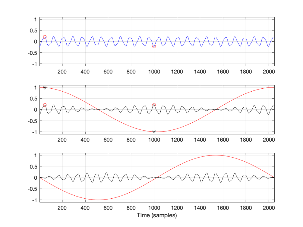
The top blue plot in Figure 4 shows the same thing that it showed in Figure 3 – it’s the 2048 samples in the recording, with sample numbers 47 and 1000 highlighted with red circles.
Take a look at the middle plot. The red curve in that plot is a cosine wave with a period (the amount of time it takes to complete 1 cycle) of 2048 samples. On that plot, I’ve put two * signs (“asterisks”, if you prefer…) – one on sample number 47 and the other at sample 1000.
One small, but important note here: although it’s impossible to see in that plot, the last value of the cosine wave is not the same as the first – it’s just a little lower in level. This is because the cosine wave would start to repeat itself on the next sample. So, the 2049th sample is equal to the 1st. This makes the period of the cosine wave 2048 samples.
The black curve in this plot is the result when you multiply the original recording (in blue) by the cosine curve (in red). So, for example, sample #47 on the blue curve (a value of 0.2054) multiplied by sample #47 on the red cosine curve (0.9901) equals 0.2033, which is indicated by a red circle on the black curve in the middle plot.
If you look at sample 1000, the value on the blue curve is positive, but when it’s multiplied by the negative value on the cosine curve, the result is a negative value on the black curve.
You’ll also notice that, when the cosine wave is 0, the result of the multiplication in the black curve is also 0.
So, we take each of the 2048 samples in the original recording of the bell, and multiply each of those values, one by one, by their corresponding samples in the cosine curve. This gives us 2048 sample values shown in the black curve, which we add all together, and that gives us a total of 1.5891.
We then do exactly the same thing again, but instead of using a cosine wave, we use a negative sine wave, shown as the red curve in the bottom plot. The blue curve multiplied by the negative sine wave, sample-by-sample results in the black curve in the bottom plot. We add all those sample values together and we get -2.5203.
Now, we do it all again at the next frequency.

Now, the period of the cosine and the negative sine waves is 1024 samples, so they’re at two times the frequency of those shown in Figure 4. However, apart from that change, the procedure is identical. We multiply the signal by the cosine wave (sample-by-sample), add up all the results, and we get 1.3547. We multiply the signal by the negative sine wave and we get -1.025.
This procedure is repeated, increasing the frequency of the cosine (the real) and the negative sine (the imaginary) waves each time. So far we have seen 0 periods (Figure 3), 1 period (Figure 2), and 2 periods (Figure 3) – we just keep going with 3 periods, 4 periods, and so on.
Eventually we get to 1024 periods. If I were to plot that, it would not look like a cosine wave, since the values would be 1, -1, 1, -1…. for 2048 samples. (But, due to the nature of digital audio and smoothing filters that we’re not going to talk about, it would, in fact, be a cosine wave at a frequency of one half of the sampling rate…)
At that frequency, the values for the negative sine wave would be a string of 2048 zeros – exactly as it is in Figure 3.
If we keep going up, we get to 2048 periods – one period of the cosine wave for each sample. This means that, at each sample, the cosine starts, so the result is a string of 2048 ones. Similarly, the negative sine wave will be a string of 2048 zeros. Note that both of these are identical to what we saw in Figure 1 when we were looking at 0 Hz…
Since we’ve already seen in the previous posting that, at a given frequency, the cosine component (the total sum of the results of multiplying the original signal by a cosine wave) is the real component and the negative sine is the imaginary component, then we can write all of the results as follows:
frequency “x”: Real + Imaginary contributions
f1: 2.9057 + 0.0000 j
f2: 1.5891 – 2.5203 j
f3: 1.3547 – 1.0251 j
…
f2047: 1.3547 – 1.0251 j
f2048: 1.5891 – 2.5203 j
f2049: 2.9057 + 0.0000 j
… and, as we saw in Figure 1 in the last post, for any one frequency, the real and imaginary contributions can be converted into a magnitude (a level) by using a little Pythagoras:
magnitude = sqrt(real^2 + imag^2)
So, we get the following magnitudes
frequency “x”: magnitude
f1: 2.9057
f2: 2.9794
f3: 1.6988
…
f2047: 1.6988
f2048: 2.9794
f2049: 2.9057
Let’s plot the first 10 values – f1 up to f10. (Remember that these are not in Hertz – they’re frequency numbers. We’ll find out what the actual frequencies are later…)

So, Figure 6 shows the beginning of the results of our calculations – the first 10 values of the 2048 values that we’re going to get. Not much interesting here yet, so let’s plot all 2048 values.
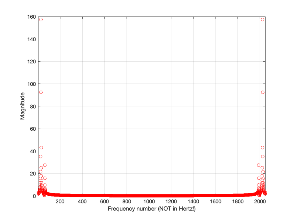
Figure 7 shows two interesting things. The first is that at least one of those numbers gets very big – almost up to 160 – whatever that means. The other is that, you may notice that we have some symmetry going on here. In fact, you might have already noticed this… If you go back and look at the lists of numbers I gave earlier, you’ll see that the values for f1 and f2049 are identical (this is true in the complex world, where we see the real and imaginary components separately, and also therefore in their magnitudes). Similarly, f2 and f2048 are identical, as are f3 and f2047. If I had put in all of the values, you would have seen that the symmetry started at f1024 which is identical to f1026. (See this posting for a discussion about aliasing, which may help to understand why this happens….)
So, since the values are repeated, we only need to look at the first 1025 values that we calculated – we know that f1026 to f2048 are the same in reverse order… So, let’s plot the bottom half of Figure 7.
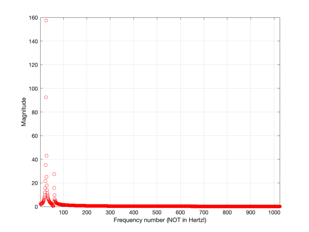
Figure 8 shows us the same information as Figure 7 – just without the symmetrical repetition. However, it’s still a little hard to read. This is because our frequency divisions are linear. Remember that we multiplied our original signal by 1 period, 2 period, 3 periods, etc… This means that we were going up in linear frequency steps – adding equal frequencies on each step. The problem is that humans hear frequency steps logarithmically – semitones (1.06 times the frequency) and octaves (2 times the frequency) are examples – we multiply (not add) in equal steps. So, let’s plot Figure 8 again, but change the X-axis to a logarithmic scale.
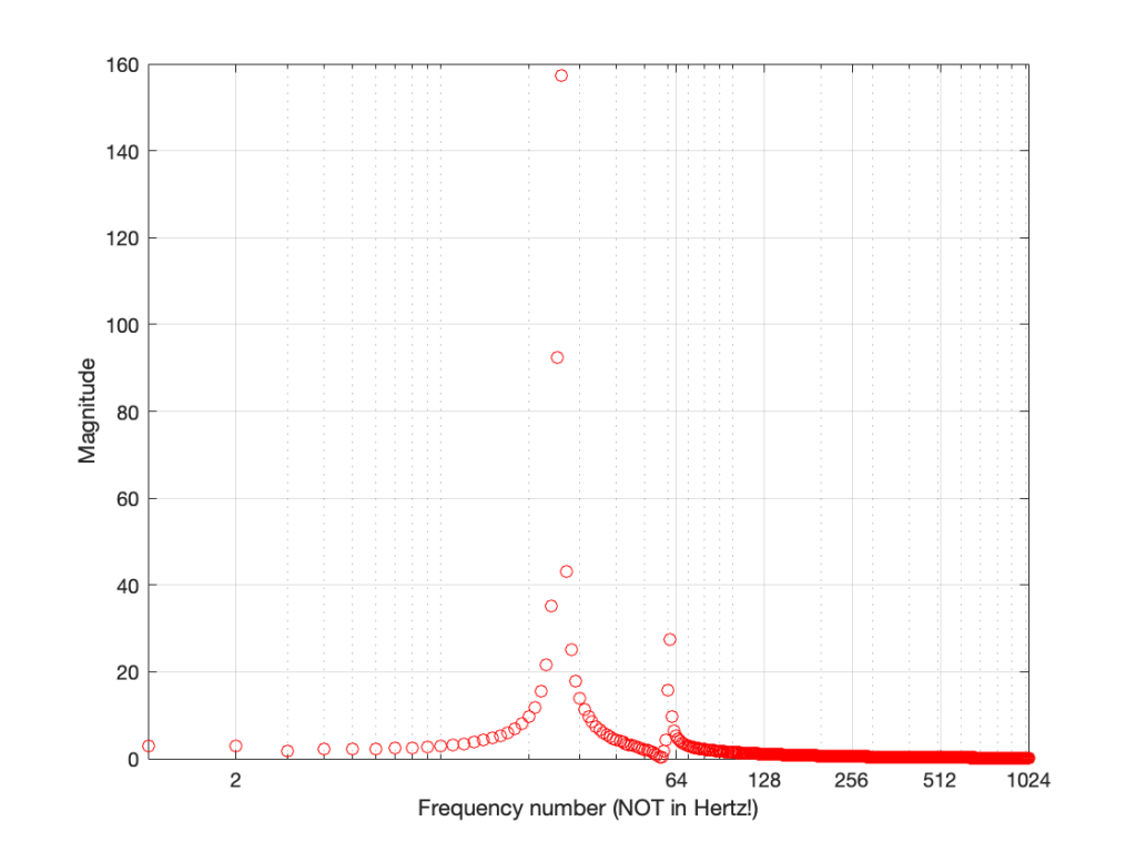
Figure 9 and Figure 8 show exactly the same information – I’ve just changed the way the x-axis is scaled so that it looks more like the way we hear distribution of frequency.
But what frequency is it?
There are two remaining problems with Figure 9 – the scaling of the two axes. Let’s tackle the X-axis first.
We know that, to get the value for f1, we found the average of all of the values in the recording. This told us the magnitude of the 0Hz. component of the signal.
Then things got a little complicated. To find the magnitude at f2, we multiplied the signal by a cosine (and a negative sine) with a period of 2048 sample. What is the frequency of that cosine wave in real life? Well, we know that the original recording was done with a sampling rate of 48 kHz or 48,000 samples per second, and our 2048-sample long slice of time equalled 42.66666666… milliseconds. If we divide the sampling rate by the period of the cosine wave, we’ll find its frequency, since we’ll find out how many times per second (per 48,000 samples) the wave will occur.
f2 = 48,000 / 2048 = 23.4375 Hz
The next frequency value will be the sampling rate divided the period of the next cosine wave – half the length of the first, or:
f3 = 48,000 / (2048 / 2) = 46.875 Hz
You might notice that f3 = 2 * f2… this helps the math.
f4 = 48,000 / (2048 / 3) = 70.3125 Hz
or f4 = 3 * f2
So, I can now keep going up to find all of my frequencies, and then change the labels on my X-axis so that they make sense to humans.

That’s one problem solved. We now know that the bell’s loudest frequency is just under 600 Hz (the peak with a magnitude of about 160) and there’s another frequency at about 1500 Hz as well – with a magnitude of about 30 or so.
But how loud is it?
So, let’s tackle the second problem – what does a magnitude of 160 mean in real life?
Not only do humans hear changes in frequency logarithmically, we also hear changes in level logarithmically as well. We say something like “a trumpet is twice as loud as a dog barking” instead of “the loudness of a trumpet is the loudness of a dog barking plus 2”. In fact, that second one just sounds silly when you say it…
As a result, we use logarithms to convert linear levels (like the ones shown on the Y-axis of Figure 10) to something that makes more sense. Instead of having values like 1, 10, 100, and 1000 (I multiplied by 10 each time), we take the log of those values, and tell people that…
Log10 (1) = 0
Log10 (10) = 1
log10 (100) = 2
log10 (1000) = 3
Now we can use the numbers on the right of those equations, which are small-ish instead of the other ones, which are big-ish…
We use this logarithmic conversion in the calculation of a decibel – which we will not get into here – but it would make the topic of another posting in the future. For now, you’ll just have to hang on…
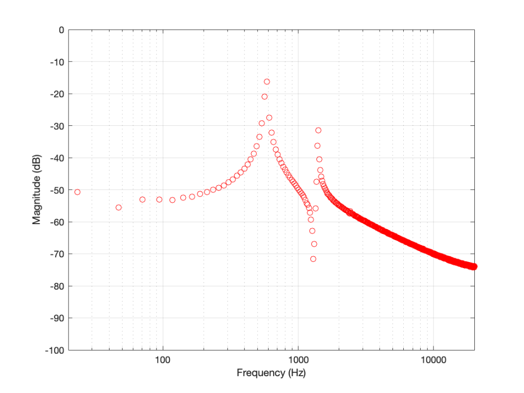
What we’ll do is to take the magnitude values plotted in Figure 10 and find their logarithms, multiply those by 20, and we get their values in decibels. Cool.
The only problem is that if I were to do that, the numbers would look unusually big. This is because I left out one step way up at the top. Back when we were multiplying and adding all those samples and cosine (and negative sine) waves, we should have done one more thing. We should have found the average value instead of the total sum. This means that we should have divided by the total number of samples. However, since we’re only looking at half of the data (the lower 1025 frequency bins – and not all 2048) we divide by half of the number of samples in our slice of time.
So, we take each sample in the recording, multiply each of those by a value in the cosine (or negative sine) wave – and divide the results by half of the number of samples. When you get that average, you then find its logarithm (base 10) and multiply by 20.
If you do that for each value, you get the result shown below in Figure 11.
If we connect the dots, then we get Figure 12.
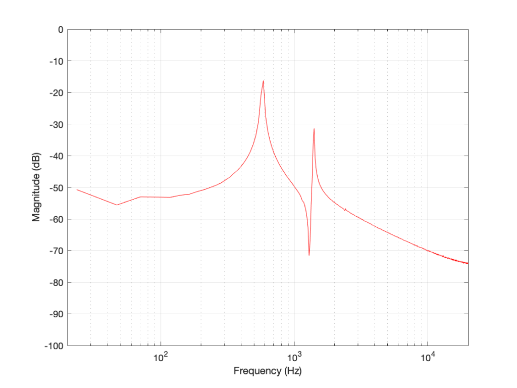
And there are the peaks we saw earlier. One just under 600 Hz at about -16 dB FS, and the other at about 1500 Hz with a level of about -31 dB FS.
The important stuff to remember for now…
There are two important things to remember from this posting.
- The frequencies that are calculated using a DFT (or FFT) are linearly spaced. That means that (on a human, logarithmic scale) we have a poor resolution in the low frequencies and a very fine resolution in the high frequencies. (for example, in this case, the first three frequencies are 0 Hz, 23.4 Hz, and 46.9 Hz. The last three frequencies are 23953.1 Hz, 23976.6 Hz, and 24,000 Hz.)
- If you want better resolution in the low frequencies, you’ll need to calculate with more samples – a longer slice of time, which means more might have happened in that time (although there are some tricks we can play, as we’ll see later).
And, you should be left with a question… Why does that plot in Figure 12 look like it’s got lots of energy at a bunch of frequencies – not just two clean spikes? We’ll get into that in the next posting: DFT’s Part 4: The Artefacts.
Human Echolocation
Closeup on vinyl
DFT’s Part 2: It’s a little complex…
Links to:
DFT’s Part 1: Some introductory basics
Whole Numbers and Integers
Once upon a time you learned how to count. You were probably taught to count your fingers… 1, 2, 3, 4 and so on. Although no one told you so at the time, you were being taught a set of numbers called whole numbers.
Sometime after that, you were probably taught that there’s one number that gets tacked on before the ones you already knew – the number 0.
A little later, sometime after you learned about money and the fact that we don’t have enough, you were taught negative numbers… -1, -2, -3 and so on. These are the numbers that are less than 0.
That collection of numbers is called integers – all “countable” numbers that are negative, zero and positive. So the collection is typically written
… -5, -4, -3, -2, -1, 0, 1, 2, 3, 4, 5 …
Rational Numbers
Eventually, after you learned about counting and numbers, you were taught how to divide (the mathematical word for “sharing equally”). When someone said “20 divided by 5 equals 4” then they meant “if you have 20 sticks, then you could put those sticks in 4 piles with 5 sticks in each pile.” Eventually, you learned that the division of one number by another can be written as a fraction like 3/1 or 20/5 or 5/4 or 1/3.
If you do that division the old-fashioned way, you get numbers like this:
3 ∕ 1 = 3.000000000 etc…
20 ∕ 5 = 4.00000000 etc…
5 ∕ 4 = 1.200000000 etc…
1 ∕ 3 = 0.333333333 etc…
The thing that I’m trying to point out here is that eventually, these numbers start repeating sometime after the decimal point. These numbers are called rational numbers.
Irrational Numbers
What happens if you have a number that doesn’t start repeating, no matter how many numbers you have? Take a number like the square root of 2 for example. This is a number that, when you multiply it by itself, results in the number 2. This number is approximately 1.4142. But, if we multiply 1.4142 by 1.4142, we get 1.99996164 – so 1.4142 isn’t exactly the square root of 2. In fact, if we started calculating the exact square root of 2, we’d result in a number that keeps going forever after the decimal place and never repeats. Numbers like this (π is another one…) that never repeat after the decimal are called irrational numbers
Real Numbers
All of these number types – rational numbers (which includes integers) and irrational numbers fall under the general heading of real numbers. The fact that these are called “real” implies immediately that there is a classification of numbers that are “unreal” – but we’ll get to that later…
Imaginary Numbers
Let’s think about the idea of a square root. The square root of a number is another number which, when multiplied by itself is the first number. For example, 3 is the square root of 9 because 3*3 = 9. Let’s consider this a little further: a positive number muliplied by itself is a positive number (for example, 4*4 = 16… 4 is positive and 16 is also positive). A negative number multiplied by itself is also positive (i.e. –4*-4 = 16).
Now, in the first case, the square root of 16 is 4 because 4*4 = 16. (Some people would be really picky and they’ll tell you that 16 has two roots: 4 and -4. Those people are slightly geeky, but technically correct.) There’s just one small snag – what if you were asked for the square root of a negative number? There is no such thing as a number which, when multiplied by itself results in a negative number. So asking for the square root of -16 doesn’t make sense. In fact, if you try to do this on your calculator, it’ll probably tell you that it gets an error instead of producing an answer.
For a long time, mathematicians just called the square root of a negative number “imaginary” since it didn’t exist – like an imaginary friend that you had when you were 2… However, mathematicians as a general rule don’t like loose ends – they aren’t the type of people who leave things lying around… and having something as simple as the square root of a negative number lying around unanswered got on their nerves.
Then, in 1797, a Norwegian surveyor named Casper Wessel presented a paper to the Royal Academy of Denmark that described a new idea of his. He started by taking a number line that contains all the real numbers like this:

He then pointed out that multiplying a number by -1 was the same as rotating by an angle of 180º, like this:
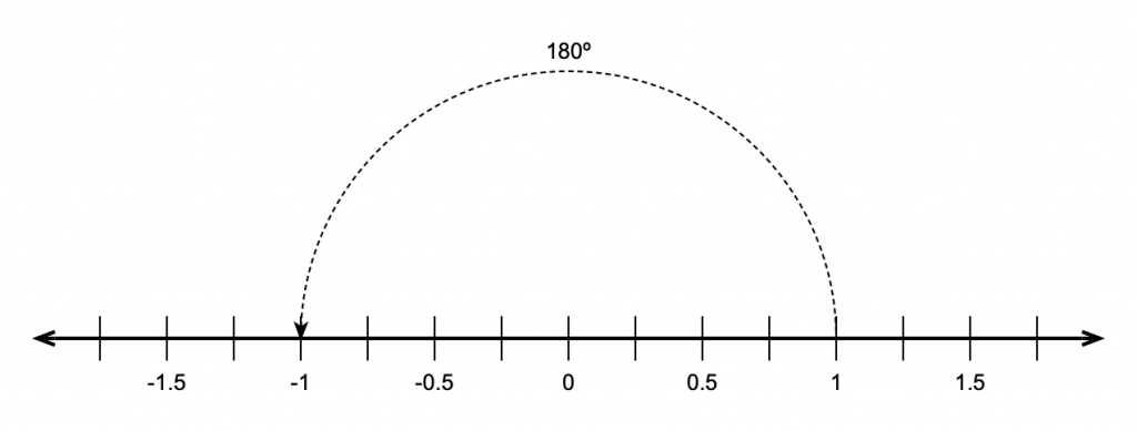
He then reasoned that, if this were true, then the square root of -1 must be the same as rotating by 90º.
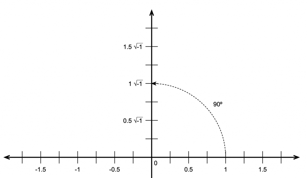
This meant that the number line we started with containing the real numbers is the X-axis on a 2-dimensional plane where the Y-axis contains the imaginary numbers. That plane is called the Z plane, where any point (which we’ll call ‘Z’) is the combination of a real number (X) and an imaginary number (Y).
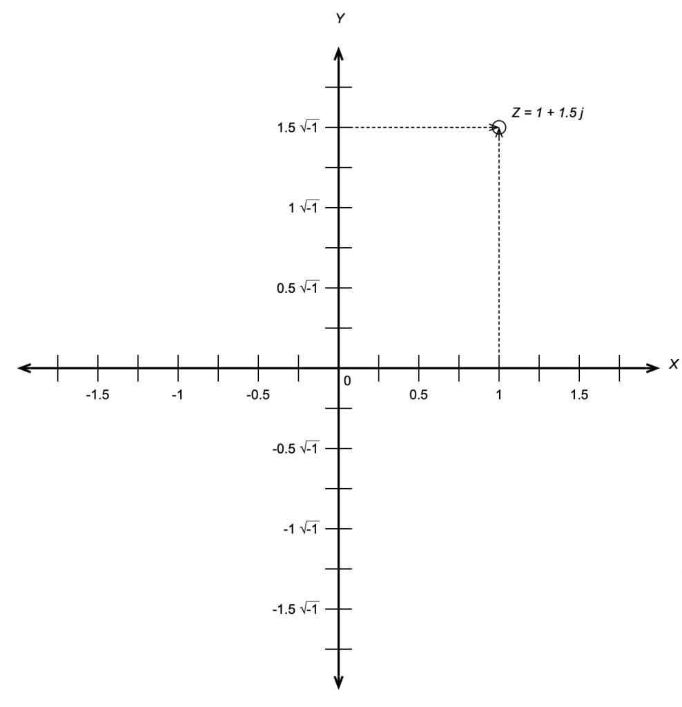
If you look carefully at Figure 4, you’ll see that I used a “j” to indicate the imaginary portion of the number. Generally speaking, mathematicians use i and physicists and engineers use j so we’ll stick with j. (The reason physics and engineering people use j is that they use i to mean “electrical current”.)
“What is j?” I hear you cry. Well, j is just the square root of -1. Of course, there is no number that is the square root of -1

and therefore

Now, remember that j * j = -1. This is useful for any square root of any negative number, you just calculate the square root of the number pretending that it was positive, and then stick a j after it. So, since the square root of 16, abbreviated sqrt(16) = 4 and sqrt(-1) = j, then sqrt(-16) = 4j.
Complex numbers
Now that we have real and imaginary numbers, we can combine them to create a complex number. Remember that you can’t just mix real numbers with imaginary ones – you keep them separate most of the time, so you see numbers like
3+2j
This is an example of a complex number that contains a real component (the 3) and an imaginary component (the 2j). In some cases, these numbers are further abbreviated with a single Greek character, like α or β, so you’ll see things like
α = 3+2j
In other cases, you’ll see a bold letter like the following:
Z = 3+2j
A lot of people do this because they like reserving Greek letters like α and ϕ for variables associated with angles.
Personally, I like seeing the whole thing – the real and the imaginary components – no reducing them to single Greek letters (they’re for angles!) or bold letters.
Absolute Value (aka the Modulus)
The absolute value of a complex number is a little weirder than what we usually think of as an absolute value. In order to understand this, we have to look at complex numbers a little differently:
Remember that j*j = -1.
Also, remember that, if we have a cosine wave and we delay it by 90º and then delay it by another 90º, it’s the same as inverting the polarity of the cosine, in other words, multiplying the cosine by -1. So, we can think of the imaginary component of a complex number as being a real number that’s been rotated by 90º, we can picture it as is shown in the figure below.
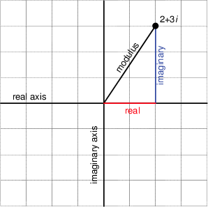
Notice that Figure 5 actually winds up showing three things. It shows the real component along the x-axis, the imaginary component along the y-axis, and the absolute value or modulus of the complex number as the hypotenuse of the triangle. This is shown in mathematical notation in exactly the same way as in normal math – with vertical lines. For example, the modulus of 2+3j is written |2+3j|
This should make the calculation for determining the modulus of the complex number almost obvious. Since it’s the length of the hypotenuse of the right triangle formed by the real and imaginary components, and since we already know the Pythagorean theorem then the modulus of the complex number (a + b j) is

Given the values of the real and imaginary components, we can also calculate the angle of the hypotenuse from horizontal using the equation


This will come in handy later.
Complex notation or… Who cares?
This is probably the most important question for us. Imaginary numbers are great for mathematicians who like wrapping up loose ends that are incurred when a student asks “what’s the square root of -1?” but what use are complex numbers for people in audio? Well, it turns out that they’re used all the time, by the people doing analog electronics as well as the people working on digital signal processing. We’ll get into how they apply to each specific field in a little more detail once we know what we’re talking about, but let’s do a little right now to get a taste.
In the previous posting, that introduces the trigonometric functions sine and cosine, we looked at how both functions are just one-dimensional representations of a two-dimensional rotation of a wheel. Essentially, the cosine is the horizontal displacement of a point on the wheel as it rotates. The sine is the vertical displacement of the same point at the same time. Also, if we know either one of these two components, we know:
- the diameter of the wheel and
- how fast it’s rotating
but we need to know both components to know the direction of rotation.
At any given moment in time, if we froze the wheel, we’d have some contribution of these two components – a cosine component and a sine component for a given angle of rotation. Since these two components are effectively identical functions that are 90º apart (for example, a cossine wave is the same as a sine that’s been delayed by 90º) and since we’re thinking of the real and imaginary components in a complex number as being 90º apart, then we can use complex math to describe the contributions of the sine and cosine components to a signal.
Huh?
Let’s look at an example. If the signal we wanted to look at a signal that consisted only of a cosine wave, then we’d know that the signal had 100% cosine and 0% sine. So, if we express the cosine component as the real component and the sine as the imaginary, then what we have is:
1 + 0 j
If the signal were an upside-down cosine, then the complex notation for it would be (–1 + 0 j) because it would essentially be a cosine * -1 and no sine component. Similarly, if the signal was a sine wave, it would be notated as (0 – 1 j).
This last statement should raise at least one eyebrow… Why is the complex notation for a positive sine wave (0 – 1 j)? In other words, why is there a negative sign there to represent a positive sine component? (Hint – we want the wheel to turn clockwise… and clocks turn clockwise to maintain backwards compatibility with an earlier technology – the sundial. So, we use a negative number because of the direction of rotation of the earth…)
This is fine, but what if the signal looks like a sinusoidal wave that’s been delayed a little? As we saw in the previous posting, we can create a sinusoid of any delay by adding the cosine and sine components with appropriate gains applied to each.
So, is we made a signal that were 70.7% sine and 70.7% cosine. (If you don’t know how I arrived that those numbers, check out the previous posting.) How would you express this using complex notation? Well, you just look at the relative contributions of the two components as before:
0.707 – 0.707 j
It’s interesting to notice that, although this is actually a combination of a cosine and a sine with a specific ratio of amplitudes (in this case, both at 0.707 of “normal”), the result will look like a sine wave that’s been shifted in phase by -45º (or a cosine that’s been phase-shifted by 45º). In fact, this is the case – any phase-shifted sine wave can be expressed as the combination of its sine and cosine components with a specific amplitude relationship.
Therefore (again), any sinusoidal waveform with any phase can be simplified and expressed as its two elemental components, the gains applied to the cosine (or real) and the sine (or imaginary). Once the signal is broken into these two constituent components, it cannot be further simplified.
DFT’s Part 1: Some introductory basics
This is the first posting in a 6-part series on doing and understanding Fourier Transforms – specifically with respect to audio signals in the digital domain. However, before we dive into DFT’s (more commonly knowns as “FFT’s”, as we’ll talk about in the next posting) we need to get some basic concepts out of the way first.
Frequency
When a normal person says “frequency” they mean “how often something happens”. I go to the dentist with a frequency of two times per year. I eat dinner with a frequency of one time per day.
When someone who works in audio says “frequency” they mean something like “the number of times per second this particular portion of the audio waveform repeats – even if it doesn’t last for a whole second…”. And, if we’re being a little more specific, then we are a bit more effuse than saying “this particular portion”… but I’m getting ahead of myself.
Let’s take a wheel with an axel, and a handle sticking out of it on its edge, like this:

We’ll turn the wheel clockwise, at a constant speed, or “frequency of rotation” – with some number of revolutions per second. If we look at the wheel from the “front” – its face – then we’ll see something like this:

When we look at the front of the wheel, we can tell its diameter (the “size” of the wheel), the frequency at which it’s rotating (in revolutions or cycles per second), and the direction (clockwise or anti-clockwise).
One way to look at the rotation is to consider the position of the handle – the red circle above – as an angle. If it started at the “3 o’clock” position, and it’s rotating clockwise, then it rotated 90 degrees when it’s at the “6 o’clock” position, for example.
However, another way to think about the movement of the handle is to see it as simultaneously moving up and down as it moves side-to-side. Again, if it moves from the 3 o’clock position to the 6 o’clock position, then it moved downwards and to the left.
We can focus on the vertical movement only if we look at the side of the wheel instead of its face, as shown in the right-hand side of the animation below.

The side-view of the wheel in that animation tells us two of the three things we know from the front-view. We can tell the size of the wheel and the frequency of its rotation. However, we don’t know whether the wheel is turning clockwise or anti-clockwise. For example, if you look at the animation below, the two side views (on the right) are identical – but the two wheels that they represent are rotating in opposite directions.

So, if you’re looking only at the side of the wheel, you cannot know the direction of rotation. However, there is one possibility – if we can look at the wheel from the side and from above at the same time, then we can use those two pieces of information to know everything. This is represented in the animation below.

Although I haven’t shown it here, if the wheel was rotating in the opposite direction, the side view would look the same, but the top view would show the opposite…
If we were to make a plot of the vertical position of the handle as a function of time, starting at the 3 o’clock position, and rotating clockwise, then the result would look like the plot below. It would start at the mid-point, start moving downwards until the handle had rotated with a “phase shift” of 90 degrees, then start coming back upwards.

If we graph the horizontal position instead, then the plot would look like the one below. The handle starts on the right (indicated as the top of the plot), moves towards the mid-point until it gets all the way to the left (the bottom of this plot) when then wheel has a phase shift (a rotation) of 180 degrees.

If we were to put these two plots together to make a three dimensional plot, showing the side view (the vertical position) and the top view (the horizontal position), and the time (or the angular rotation of the wheel), then we wind up with the plot shown below.

Time to name names… The plot shown in Figure 6 is a “sine wave”, plotted upside down. (The word sine coming from the same root as words like “sinuous” and “sinus” (as in “could you hand me a tissue, please… my sinuses are all blocked up…”) – from the Latin word “sinus” meaning “a bay” – as in “sittin’ by the dock of the bay, watchin’ the tide roll in…”.) Note that, if the wheel were turning anti-clockwise, then it would not be upside down.
Phase
If you look at the plot in Figure 7, you may notice that it looks the same as a sine wave would look, if it started 90 degrees of rotation later. This is because, when you’re looking at the wheel from the top, instead of the side, then you have rotated your viewing position by 90 degrees. This is called a “cosine wave” (because it’s the complement of the sine wave).
Notice how, whenever the sine wave is at a maximum or a minimum, the cosine wave is at 0 – in the middle of its movement. The opposite is also true – whenever the cosine is at a maximum or a minimum, the sine wave is at 0.
Remember that if we only knew the cosine, we still wouldn’t know the direction of rotation of the wheel – we need to know the simultaneous values of the sine and the cosine to know whether the wheel is going clockwise or counterclockwise.
The important thing to know so far is that a sine wave (or a cosine wave) is just a two-dimensional view of a three-dimensional thing. The wheel is rotating with a frequency of some angle per second (one full revolution per second = 360º/sec. 10 revolutions per second = 3600º/sec) and this causes a point on its circumference (the handle in the graphics above) to move back and forth (along the x-axis, which we see in the “top” view) and up and down (along the y-axis, which we see in the side view).
So what?
Let’s say that I asked you to make a sine wave generator – and I would like the wave to start at some arbitrary phase. For example, I might ask you to give me a sine wave that starts at 0º. That would look like this:

But, since I’m whimsical, I might say “actually, can you start the sine wave at 45º instead please?” which would look like this:

One way for you do do this is to make a sine wave generator with a very carefully timed gain control after it. So, you start the sine wave generator with its output turned completely down (a gain of 0), and you wait the amount of time it takes for 45º of rotation (of the wheel) to elapse – and then you set the output gain suddenly to 1.
However, there’s an easier way to do it – at least one that doesn’t require a fancy timer…
If you add the values of two sinusoidal waves of the same frequency, the result will be a sinusoidal waveform with the same frequency. (There is one exception to this statement, which is when the two sinusoids are 180º apart and identical in level – then if you add them, the result is nothing – but we’ll forget about that exception for now…)
This also means that if we add a sine and a cosine of the same frequency together (remember that a cosine wave is just a sine wave that starts 90º later) then the result will be a sinusoidal waveform of the same frequency. However, the amplitude and the phase of that resulting waveform will be dependent on the amplitudes of the sine and the cosine that you started with…
Let’s look at a couple of examples of this.

Figure 11, above shows that if you take a cosine wave with a maximum amplitude of 0.7 (in blue) and a sine wave of the same frequency and amplitude, starting at a phase of 180º (or -1 * the sine wave starting at 0º), and you add them together (just add their “y” values, for each point on the x axis – I’ve shown this for an X value of 270º in the figure), then the result is a cosine wave with an amplitude of 1 and a phase delay of 45º (or a sine wave with a phase delay of 135º (45+90 = 135) – it’s the same thing…)
Here’s another example:

In Figure 12 we see that if we add a a cosine wave * -0.5 and add it to a sine wave * -0.866, then the result is a cosine wave with an amplitude of 1, starting at 120º.
I can keep doing this for different gains applied to the cosine and sine wave, but at this point, I’ll stop giving examples and just say that you’ll have to trust me when I say:
If I want to make a sinusoidal waveform that starts at any phase, I just need to add a cosine and a sine wave with carefully-chosen gains…
Pythagoreas gets involved…
You may be wondering how I found the weird gains in Figures 11 and 12, above. In order to understand that, we need to grab a frame from the animation in Figure 5. If we do that, then you can see that there’s a “hidden” right triangle formed by the radius of the wheel, and the vertical and the horizontal displacement of the handle.

Pythagoras taught us that the square of the hypotenuse of a right triangle is equal to the sum of the squares of the two other sides. Or, expressed as an equation:
a2 + b2 = c2
where “c” is the length of the hypotenuse, and “a” and “b” are the lengths of the other two sides.
This means that, looking at Figure 13:
cos2(a) + sin2(a) = R2
I’ve set “R” (the radius of the wheel ) to equal 1. This is the same as the amplitude of the sum of the cosine and the sine in Figures 11 and 12… and since 1*1 = 1, then I can re-write the equation like this:
sine_gain = sqrt ( 1 – cosine_gain2)
So, for example, in Figure 12, I said that the gain on the cosine is -0.5, and then I calculated sqrt(1 – -0.52) = 0.86603 which is the gain that I applied to the upside-down sine wave.
Three ways to say the same thing…
I can say “a sine wave with an amplitude of 1 and a phase delay of 135º” and you should now know what I mean.
I could also express this mathematically like this:

which means the value of y at a given value of α is equal to A multiplied by the sine of the sum of the values α and ϕ. In other words, the amplitude y at angle α equals the sine of the angle α added to a constant value ϕ and the peak value will be A. In the above example, y(α) would be equal to 1*sin(α +135∘) where α can be any value depending on the time (because it’s the angle of rotation of the wheel).
But, now we know that there is another way to express this. If we scale the sine and cosine components correctly and add them together, the result will be a sinusoidal wave at any phase and amplitude we want. Take a look at the equation below:

where A is the amplitude
ϕ is the phase angle
α is any angle of rotation of the wheel
a = Acos(ϕ)
b = Asin(ϕ)
What does this mean? Well, all it means is that we can now specify values for a and b and, using this equation, wind up with a sinusoidal waveform of any amplitude and phase that we want. Essentially, we just have an alternate way of describing the waveform.
In Part 2, we’ll talk about a fourth way of saying the same thing…

