This past week I found a very small oddity in the behaviour of one of the functions in Matlab. This led me down a rabbit hole that I’m still following, but the stuff I’ve learned along the way has proven to be interesting.

The summary

The short version of the story is that I made a test tone which consisted of a sine wave that had a frequency that matched an FFT bin centre so that I could test a thing. In order to get the sine wave through the thing, I had to export the audio signal as something the thing could play. So, I exported it as both a .wav and a .flac file, both with 24-bit word lengths and matching sampling rates.

Once the two signals came back from the thing, they looked different on an FFT analysis. Not very different, but different enough to raise questions. So, I ran the FFT on the .wav and .flac files that I created to do the test and found out that THEY were different, which I didn’t expect, because I know that FLAC is lossless.

The question that came up first was “why are they different?”, and that was just the entrance to the rabbit hole.

The long version

In order to explain what happened, we have to following some advice given by Carl Sagan who said

‘If you wish to make an apple pie from scratch, you must first invent the universe.’

We won’t invent the universe, but we’re going to dig down into the basics of LPCM digital audio in order to come back up to talk about where I wound up last Thursday.

Quantisation

Linear Pulse Code Modulation (LPCM) is a way of encoding signals (like an audio signal) by saving the waveform as a series of measurements of the instantaneous amplitude. However, when you do this, you can’t have a measurement with an infinite resolution, so you have to round off the value to the nearest one you can encode. This is just like measuring something with a ruler that has millimetres marked on it. You can’t really measuring something with a precision of less than the nearest millimetre, so you round off the value to something you know. Whether or not that’s good enough depends on what the measurement is for.

In LPCM digital audio, we call the steps that you can round the values to ‘quantisation levels’ because you’re dividing up the amplitude into discrete quanta. Since the values of those quantisation levels are stored or transmitted using a binary number (containing only 0s and 1s), the number of quantisation levels is a power of 2. For example, if you have a 16-bit (bit = Binary digIT) value, then you can count from

0000 0000 0000 0000 = 0
to
1111 1111 1111 1111 = 2¹⁶ = 65,536

However, since audio signals go above and below 0 (we need to represent positive and negative values) we need a way to split up those options above (a range of 0 to 65,536) to do this.

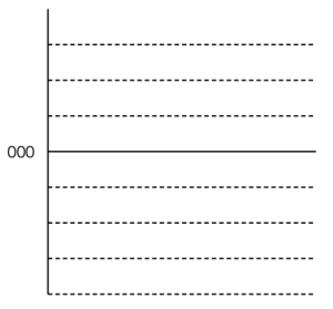
Let’s take a simple example with a 3-bit long word. Since there are 3 bits, we have 2³ = 8 quantisation levels. It would be nice if 000 in the binary representation referred to a signal value of 0, like this:

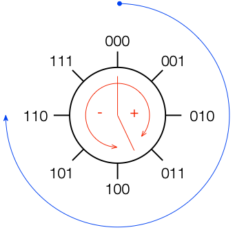
All we need to do now is to figure out what binary values to put on the other quantisation levels. To do this, we use a system like the one shown in Figure 2.

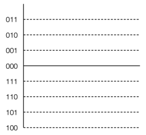
If you start at the top, and follow the blue circular arrow going clockwise, you count from 000 ( = 0) all the way to 111 (= 7). However, if you look at the red arrows, you can see that we can assign the binary values to the positive and negative quantisation levels by looking at the circle clockwise for positive values and counter-clockwise for negative ones. This means that we wind up with the assignments shown in Figure 3.

This way of using ‘wrapping’ the values around the circle into number assignments on a one-dimensional (in this case, vertical) scale is called a ‘two’s complement’ method.

There are two nice things about this system:

• the middle value of 0 is assigned an actual value of 0, which makes sense to us humans
• the first bit (digit) in the binary value tells you whether the level is positive (if it’s a 0) or negative (if it’s a 1).

There is at least one slightly annoying thing about this system: it’s asymmetrical. Notice in Figure 3 that there are 3 available positive quantisation levels, but 4 negative ones. This is because we have an even number of values to use (because it’s a power of 2) but one of the values is 0, leaving an odd, and therefore asymmetrical number of remaining values for the non-0 quantisation levels.

This will come back to be a pain in the arse later…